Artificial DEM
Computational approach
stepsize, effectively quadrupling the number of squares, while concurrently scaling down the roughness factor, which can be moderated linearly or exponentially. This iterative refinement continues until the stepsize reaches two, at which point the artificial DEM’s elevations are fully determined.art_DEM.generate_fractal_map() function, facilitating the overlay of coarser topographic features with finer details. To mimic the typical slopes found in volcanic regions, a routine has been crafted to impose a incline across the fractal map. Precision within the DEM is optimized by limiting elevation values to two decimal places, which is sufficient for representing the terrain while significantly reducing the DEM’s file size. The finalized DEM is then exported to an ASCII file using art_DEM.write_dem_to_ascii(), including essential metadata in the file header.art_DEM.generate_pathfile() function, which calculates xy-coordinates for a series of observational points situated approximately at the center of the domain.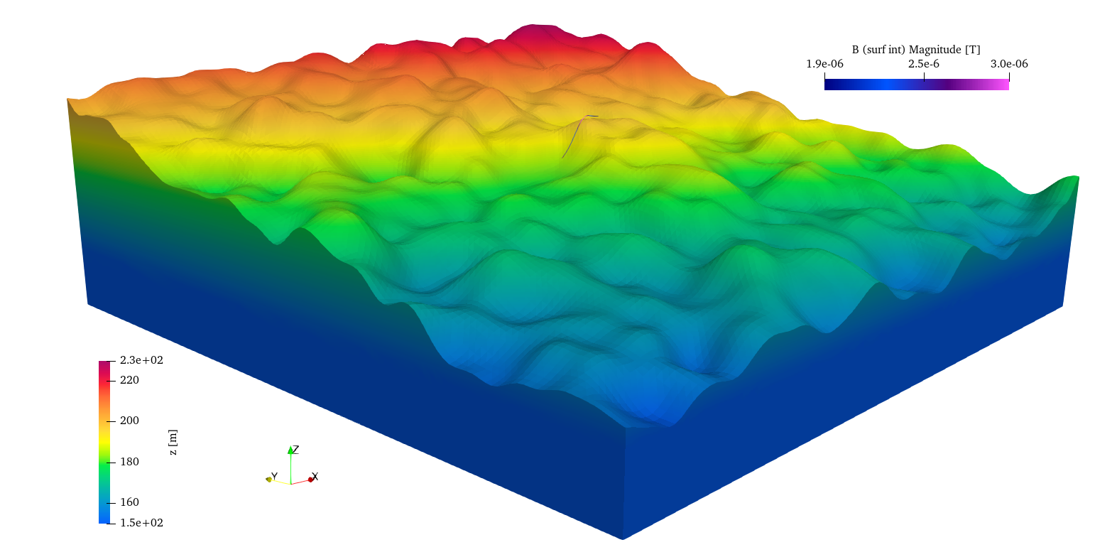
Figure 23 3D visualization of a synthetic DEM showing varied terrain roughness, generated using a fractal-based algorithm to mimic natural topographic features. In the middle of the domain is an observational path for the computation of the magnetic field B.
Model setup
Results
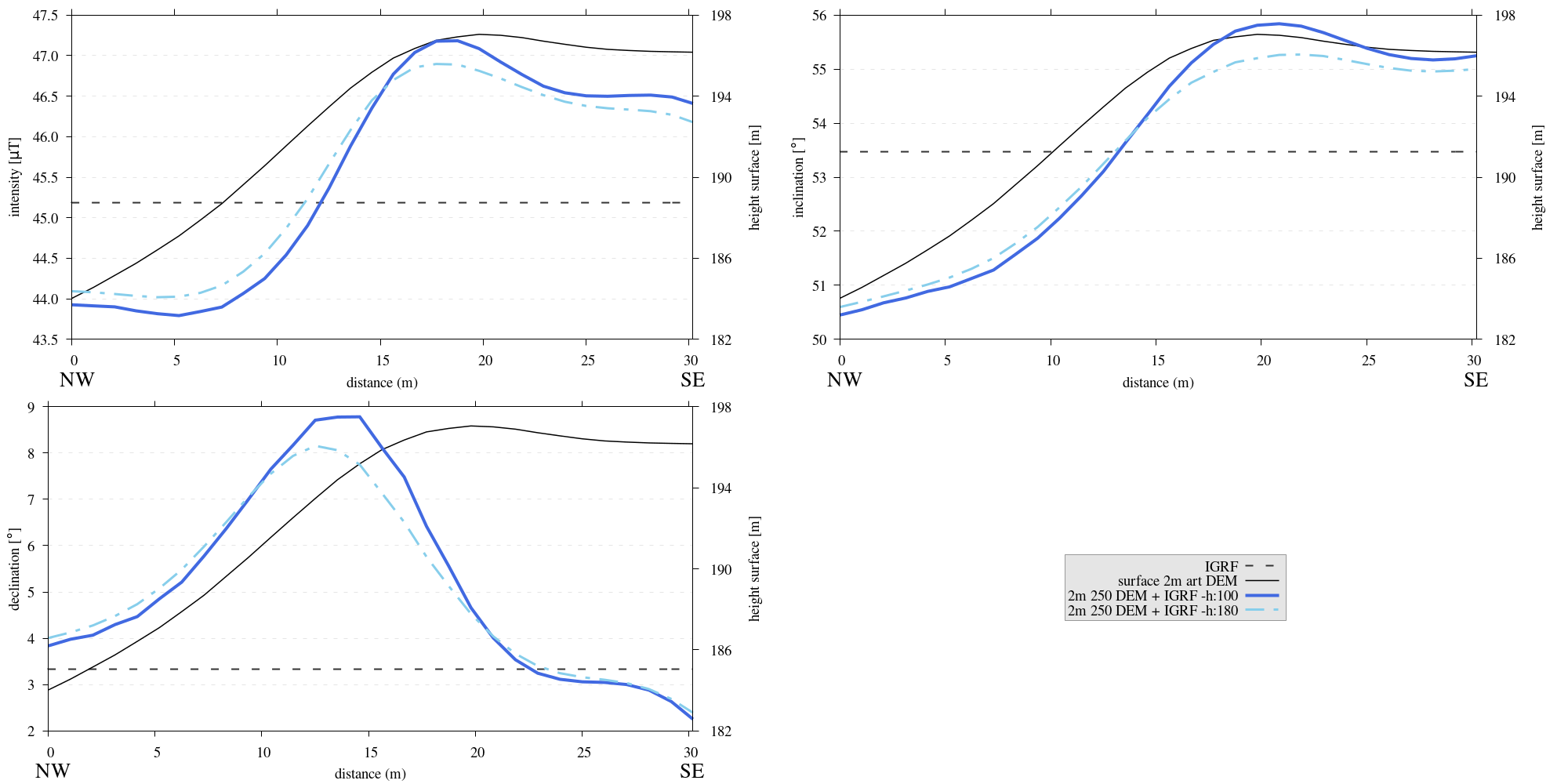
Figure 24 Three subplots depicting the intensity [\(\mu T\)], inclination [\(^{\circ}\)] and declination [\(^{\circ}\)] of the computed magnetic field B superimposed on the IGRF derived from flank simulations. Simulations are done at both \(1m\) and \(1.8m\) above the topography. Similar trends as before can be observed, the ambient magnetic field is a function of topography.
Reproduce
script_art_DEM.sh shell script has been crafted to automate the execution and organization of output data, directing it into the correct subdirectory for a run using the artificial DEM generating module art_DEM.py. Please make sure any modifications of theSteps to reproduce the results and figures
Please note basic setup in Installation
In
MTE.py, modify benchmark attribution to-1, and make sure the right setup is used:49 50 51 52 53 54 55 56 57 58 59 60 61 62 63 64 65 66 67 68 69 70 71 72 73 74 75 76 77 78 79 80
benchmark = '-1'

compute_vi = False  # This includes the volume integral computation by Gaussian quadrature, see
                    # documentation, possible for all setups apart from DEM (-1).
if compute_vi:
   nqdim = 6  # Number of quadrature points, see documentation.

## ONLY BENCHMARK = -1 (DEM) & BENCHMARK = 5 (FLANKSIM) ##
flat_bottom = True  # If True, a flat bottom is generated at the lower surface of the domain.
                    # Please see documentation, as the specific setup of this feature is different
                    # for the flank simulations and the DEM test.
remove_zerotopo = True  # Setup run 2 times: 1st time, zero topography setup: xy coordinates
                        # of the observation points the same, but zerotopo domain and obs path
                        # shifted to average height DEM. 2nd time, "regular" run with topography.
                        # final results are 2nd run - 1 st run values. Run time can be improved,
                        # if 1st run was done with less el (and cuboid function), yet to be done.

## ONLY BENCHMARK = 5 (FLANKSIM) ##
subbench = 'south'  # 'south', 'east', 'north', 'west', input parameters imported from flanksim
           # have priority over any choice made here. So if this is used, make sure to
           # comment out the import line in section below!
global_run = False

## ONLY BENCHMARK = -1 (DEM) ##
art_DEM = True  # if True, path/topo file (+ header) produced by art_DEM.py read in.
                # Please note other values specified below for IGRF and magnetization etc.

## BENCHMARK == -1 OR 5 ##
add_noise = False  # if True, noise is added to the DEM after loading in from file.
Nf = 1.5  # noise amplitude between -Nf and Nf, value added to the z-coor of the middle node
          # on the top/bottom surface. Only relevant if adding noise, increasing this value,
          # increases the amount of noise superimposed on the DEM.
In
MTE.py, fill the required parameters.325 326 327 328 329 330 331 332 333 334 335 336 337 338 339 340 341 342 343 344 345 346 347 348 349 350 351 352 353 354 355 356 357 358 359 360 361 362 363 364 365 366 367 368 369 370 371 372 373 374 375 376 377 378
if benchmark == '-1':
   # General settings ## DO NOT CHANGE ##
   compute_analytical = False
   compute_vi = False

   if art_DEM:
      # General settings
      do_line_measurements = False
      do_plane_measurements = False
      do_spiral_measurements = False
      do_path_measurements = True

      # Domain settings
      Lz = 20
      nelz = 10
      IGRFx = 26850.3e-9  # Pmag coordinate configuration!
      IGRFy = 1561.2e-9  # Mount Etna (peak)
      IGRFz = 36305.7e-9
      Mx0, My0, Mz0 = 0, 4.085, -6.29

      # Path measurement settings
      pathfile = 'sites/art_path.txt'
      print('reading from art_path.txt')
      with open(pathfile, 'r') as path:
         npath = len(path.readlines())
      zpath_height = 1  # height above topo
      ho = zpath_height

      # Domain settings from artificial DEM
      topofile = 'DEMS/art_dem.ascii'
      print('reading from art_dem.ascii')
      with open(topofile, 'r') as topo:
           has_header, header = read_header(topo)

      if has_header:
         nnx = int(header['ncols'])
         nny = int(header['nrows'])
         cellsize = header['cellsize']

         nelx = nnx - 1
         nely = nny - 1
         Lx = nelx * cellsize
         Ly = nely * cellsize
      else:  # define values here if no header is present in DEM
         nnx = 31
         nny = 31
         cellsize = 2
         xllcorner = 0
         yllcorner = 0

         nelx = nnx - 1
         nely = nny - 1
         Lx = nelx * cellsize
         Ly = nely * cellsize
In
script_art_DEM.sh, fill the required parameters.3 4 5 6 7 8 9 10 11 12 13 14 15 16 17 18 19 20 21 22 23 24
generate_DEM=true # Domain parameters ncol=127 # must be a power of 2 minus 1: 2^n - 1, e.g., 3, 7, 15, 31, 63, 127, 255, 511, 1023 ... nrow=127 # amount of rows (must be equal to amount of columns, ncol) cellsize=2 # Change this value if you want a different cell size afx=5 # angle of flank in x-direction afy=12 # angle "" in y-direction xllcorner=50 # x-coordinate of the lower left corner (most south-western node) yllcorner=100 # y-coordinate of "" sigma=2 # sigma for Gaussian filter roughness1=12 # can be adjusted for desired level of detail roughness2=2 # can be adjusted for desired level of detail # Path parameters rough_length=30 # rough length of the path, but due to shifting length might be slighlt more/less npath=30 # amount of observation points on path size=$(( (ncol - 1) * cellsize )) folder_name="${size}_r${roughness1}_r${roughness2}_afx${afx}_afy${afy}_s${sigma}"
Run DEM simulation:
./script_art_DEM.sh
Modify for 1.8 meter run:
345 346 347 348 349 350
# Path measurement settings pathfile = 'sites/art_path.txt' print('reading from art_path.txt') with open(pathfile, 'r') as path: npath = len(path.readlines()) zpath_height = 1.8 # height above topo
 3
 4
 5
 6
 7
 8
 9
10
11
12
13
14
15
16
17
18
19
20
21
22
23
24
generate_DEM=false # Domain parameters ncol=127 # must be a power of 2 minus 1: 2^n - 1, e.g., 3, 7, 15, 31, 63, 127, 255, 511, 1023 ... nrow=127 # amount of rows (must be equal to amount of columns, ncol) cellsize=2 # Change this value if you want a different cell size afx=5 # angle of flank in x-direction afy=12 # angle "" in y-direction xllcorner=50 # x-coordinate of the lower left corner (most south-western node) yllcorner=100 # y-coordinate of "" sigma=2 # sigma for Gaussian filter roughness1=12 # can be adjusted for desired level of detail roughness2=2 # can be adjusted for desired level of detail # Path parameters rough_length=30 # rough length of the path, but due to shifting length might be slighlt more/less npath=30 # amount of observation points on path size=$(( (ncol - 1) * cellsize )) folder_name="${size}_r${roughness1}_r${roughness2}_afx${afx}_afy${afy}_s${sigma}_180"
Run DEM simulation for 1.8 meter:
./script_art_DEM.sh
Go to directory and plot:
cd path_results/art_DEM/
gnuplot plot_script_art_dem.p
Adding noise to DEM
Nf parameter. It’s important to be aware that this method of noise introduction is quite basic and may lead to some unanticipated outcomes. For example, excessive noise coupled with an observation point situated near an element’s midpoint may result in the point being erroneously placed within the magnetization domain. It is advised to be cautious during the setup phase of any experiments using this function to ensure that observation points remain outside the magnetization domain, as there are no corrective measures or tests for this within the system.Results and analyses
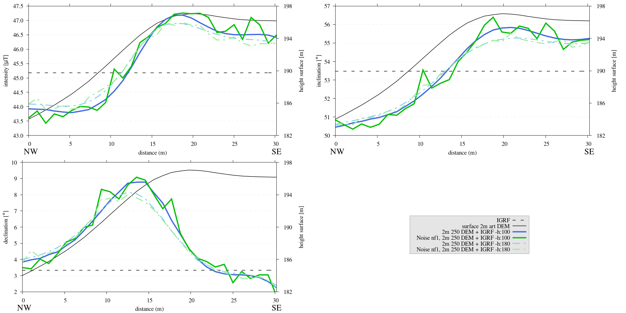
Figure 25 Three subplots depicting the intensity [\(\mu T\)], inclination [\(^{\circ}\)] and declination [\(^{\circ}\)] of the computed magnetic field B superimposed on the IGRF derived from flank simulations. These simulations are conducted at 1 meter and 1.8 meters above the terrain surface. To add variability, the midpoint of each element’s surface is altered by introducing a random noise factor ranging between -1 and 1 meter. Results show that adding noise introduces more variations and introduces frequent sudden peaks and dips in the magnetic field curves.
Reproduce
Steps to reproduce the results and figures
Please note basic setup in Installation
In
MTE.py, modify benchmark attribution to-1, and make sure the right setup is used:49 50 51 52 53 54 55 56 57 58 59 60 61 62 63 64 65 66 67 68 69 70 71 72 73 74 75 76 77 78 79 80
benchmark = '-1' compute_vi = False # This includes the volume integral computation by Gaussian quadrature, see # documentation, possible for all setups apart from DEM (-1). if compute_vi: nqdim = 6 # Number of quadrature points, see documentation. ## ONLY BENCHMARK = -1 (DEM) & BENCHMARK = 5 (FLANKSIM) ## flat_bottom = True # If True, a flat bottom is generated at the lower surface of the domain. # Please see documentation, as the specific setup of this feature is different # for the flank simulations and the DEM test. remove_zerotopo = True # Setup run 2 times: 1st time, zero topography setup: xy coordinates # of the observation points the same, but zerotopo domain and obs path # shifted to average height DEM. 2nd time, "regular" run with topography. # final results are 2nd run - 1 st run values. Run time can be improved, # if 1st run was done with less el (and cuboid function), yet to be done. ## ONLY BENCHMARK = 5 (FLANKSIM) ## subbench = 'south' # 'south', 'east', 'north', 'west', input parameters imported from flanksim # have priority over any choice made here. So if this is used, make sure to # comment out the import line in section below! global_run = False ## ONLY BENCHMARK = -1 (DEM) ## art_DEM = True # if True, path/topo file (+ header) produced by art_DEM.py read in. # Please note other values specified below for IGRF and magnetization etc. ## BENCHMARK == -1 OR 5 ## add_noise = True # if True, noise is added to the DEM after loading in from file. Nf = 1 # noise amplitude between -Nf and Nf, value added to the z-coor of the middle node # on the top/bottom surface. Only relevant if adding noise, increasing this value, # increases the amount of noise superimposed on the DEM.
In
MTE.py, fill the required parameters.345 346 347 348 349 350
# Path measurement settings pathfile = 'sites/art_path.txt' print('reading from art_path.txt') with open(pathfile, 'r') as path: npath = len(path.readlines()) zpath_height = 1 # height above topo
In
script_art_DEM.sh, fill the required parameters.3 4 5 6 7 8 9 10 11 12 13 14 15 16 17 18 19 20 21 22 23 24
generate_DEM=false # Domain parameters ncol=127 # must be a power of 2 minus 1: 2^n - 1, e.g., 3, 7, 15, 31, 63, 127, 255, 511, 1023 ... nrow=127 # amount of rows (must be equal to amount of columns, ncol) cellsize=2 # Change this value if you want a different cell size afx=5 # angle of flank in x-direction afy=12 # angle "" in y-direction xllcorner=50 # x-coordinate of the lower left corner (most south-western node) yllcorner=100 # y-coordinate of "" sigma=2 # sigma for Gaussian filter roughness1=12 # can be adjusted for desired level of detail roughness2=2 # can be adjusted for desired level of detail # Path parameters rough_length=30 # rough length of the path, but due to shifting length might be slighlt more/less npath=30 # amount of observation points on path size=$(( (ncol - 1) * cellsize )) folder_name="${size}_r${roughness1}_r${roughness2}_afx${afx}_afy${afy}_s${sigma}_noise_af1"
Run DEM simulation:
./script_art_DEM.sh
Modify for 1.8 meter run:
345
346
347
348
349
350
# Path measurement settings
pathfile = 'sites/art_path.txt'
print('reading from art_path.txt')
with open(pathfile, 'r') as path:
   npath = len(path.readlines())
zpath_height = 1.8  # height above topo
24folder_name="${size}_r${roughness1}_r${roughness2}_afx${afx}_afy${afy}_s${sigma}_noise_af1_180"Run DEM simulation for 1.8 meter:
./script_art_DEM.sh
Go to directory and plot:
cd path_results/art_DEM/
gnuplot plot_script_art_dem_noise.p
Adding another DEM
Ensure that the file locations and names of the DEM and path file are consistent between the code’s main body and the file directory.
The DEM ASCII file should adhere to a standard format, with the top-left value (below the header) representing the most northwestern point. If the DEM’s structure deviates from this norm, the code segment responsible for parsing DEM values will require modification to accommodate the alternative format.
The DEM header must include the following attributes:
ncol, nrow, xllcorner, yllcorner, cellsize. The functionsupport.read_header()will flag an error if the header is incomplete or incorrectly formatted. In the absence of a header, these attributes must be manually set within theMTE.pyscript.When incorporating published DEMs and field data, their coordinate systems must be in sync.
A common issue is the potential discrepancy between the topography from field data and that of a published DEM, particularly in the vertical dimension due to the known limitations of GPS devices in measuring elevation accurately. To account for any such height discrepancies, a path offset height (
poh) can be specified (see code snippet below), which is then subtracted from the field elevation measurements for more accurate representation and easier plotting.
It is also possible to encounter slight spatial misalignments between field measurements and the DEM. Such discrepancies are usually localized and should be assessed visually for each path.
The use of any external reference field is supported, as the
support.add_referencefield()function is designed to be universal and adaptable to various datasets.
Footnotes
- 1
This step is called the diamond step, this might sound counterintuitive, as the midpoint of the square is modified. Nonetheless, the rationale behind the nomenclature becomes clear when considering the points that contribute to determining the new value. For a comprehensive explanation and visual representation, refer to the detailed entry on the diamond-square algorithm on wikipedia.