Synthetic topopography: flank simulations
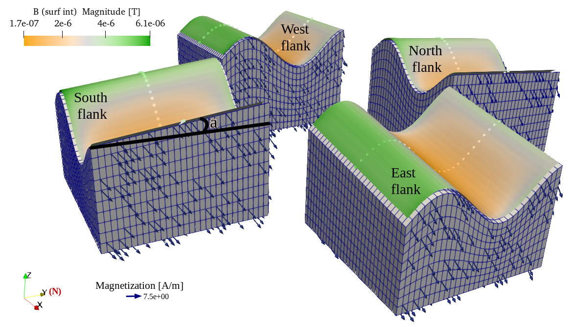
Figure 21 Flank simulation on the Etna. (\(\mathbf{M}\)) = \(7.5 [A/m]\) (arrows). The slope (\(a\) in Figure 21) is \(6 ^{\circ}\). The computations of the magnetic field (\(\mathbf{B}\)) above the flanks are done at point composing either a path or a plane above each flank. The flanks are labeled as displayed. Please note, for visual purposes, the extent and resolution of the displayed mesh do not adhere the optimized testing setup outlined before in the parameter section.
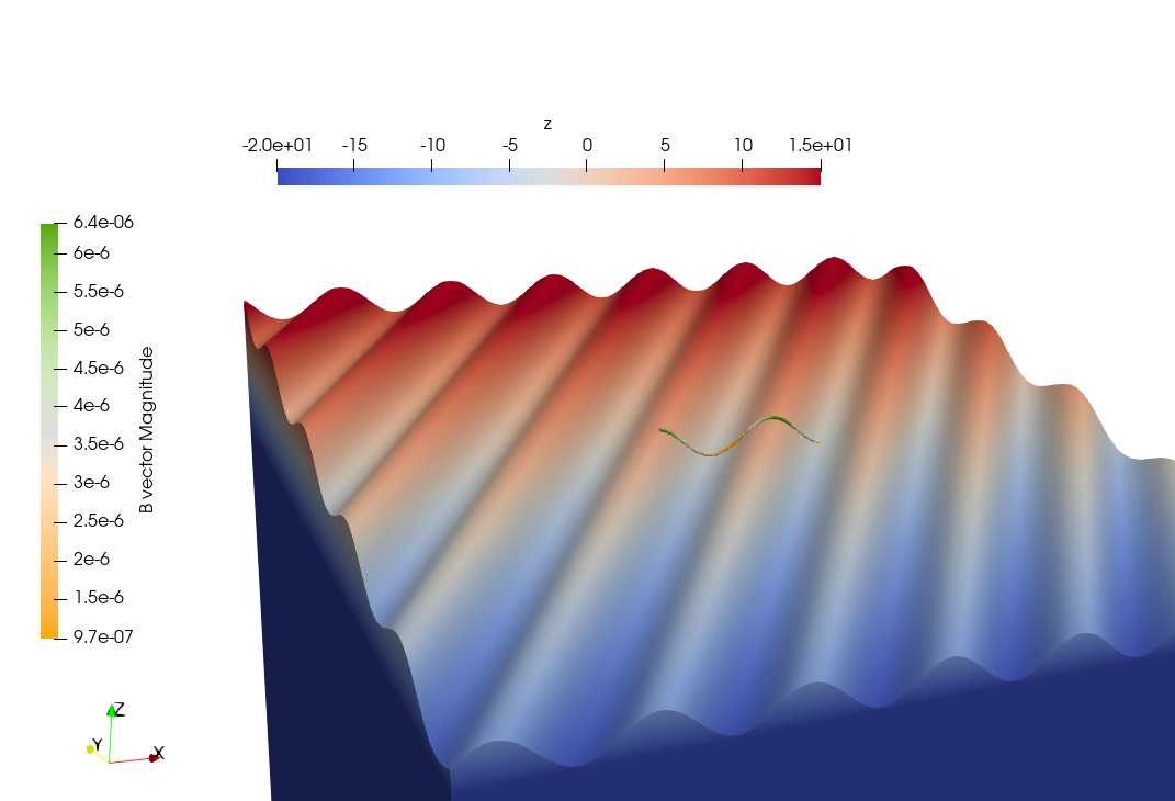
Figure 22 Direction of wavy pattern on south flank is \(-31 ^{\circ}\), an example of a variation possible while doing flank simulations tests.
Model setup
support.topography(), traverses perpendicular across the inclined surface.Reproduce
flanksim.py, has been integrated into the codebase for executing full simulations across all flanks. To activate this module, uncomment the corresponding line in the MTE.py file (see steps below). Additionally, the script_flanksim.sh shell script has been crafted to automate the execution and organization of output data, directing it into the correct subdirectory 1 for each flank simulation.Steps to reproduce the results and figures
Please note basic setup in Installation
In
MTE.py, modify benchmark attribution to5, and make sure the right setup is used & MTE.py imports fromflanksim.py():49 50 51 52 53 54 55 56 57 58 59 60 61 62 63 64 65 66 67 68 69 70
benchmark = '5'

compute_vi = False  # This includes the volume integral computation by Gaussian quadrature, see
                    # documentation, possible for all setups apart from DEM (-1).
if compute_vi:
   nqdim = 6  # Number of quadrature points, see documentation.

## ONLY BENCHMARK = -1 (DEM) & BENCHMARK = 5 (FLANKSIM) ##
flat_bottom = True  # If True, a flat bottom is generated at the lower surface of the domain.
                    # Please see documentation, as the specific setup of this feature is different
                    # for the flank simulations and the DEM test.
remove_zerotopo = True  # Setup run 2 times: 1st time, zero topography setup: xy coordinates
                        # of the observation points the same, but zerotopo domain and obs path
                        # shifted to average height DEM. 2nd time, "regular" run with topography.
                        # final results are 2nd run - 1 st run values. Run time can be improved,
                        # if 1st run was done with less el (and cuboid function), yet to be done.

## ONLY BENCHMARK = 5 (FLANKSIM) ##
subbench = 'south'  # 'south', 'east', 'north', 'west', input parameters imported from flanksim
           # have priority over any choice made here. So if this is used, make sure to
           # comment out the import line in section below!
global_run = False
231
232
233
234
235
236
237
238
239
240
241
242
243
244
245
246
247
248
249
250
251
252
253
254
255
256
257
258
259
260
261
262
if benchmark == '5':
   # General settings
   do_spiral_measurements = False
   do_path_measurements = False
   compute_analytical = False

   # Domain settings
   Lx, Ly, Lz = 250, 250, 20
   nelx, nely, nelz = int(Lx * 1.5), int(Ly * 1.5), 10
   Mx0, My0, Mz0 = 0, 4.085, -6.29
   #Lx, Ly, Lz = 50, 50, 120
   #nelx, nely, nelz = 10, 10, 10

   # Synthetic topography settings
   wavelength = 25
   A = 4
   af = 6

   # Line measurement settings
   do_line_measurements = True
   line_nmeas = 47
   xstart, xend = 0.23 + ((Lx - 50) / 2), 49.19 + ((Ly - 50) / 2)
   ystart, yend = Ly / 2 - 0.221, Ly / 2 - 0.221
   zstart, zend = 1, 1  # 1m above surface.

   # Plane measurement settings
   do_plane_measurements = False
   plane_nnx, plane_nny = 30, 30
   plane_x0, plane_y0, plane_z0 = -Lx / 2, -Ly / 2, 1
   plane_Lx, plane_Ly = 2 * Lx, 2 * Ly

   from flanksim import *
Run flank simulation:
./script_flanksim.sh
Modify for 1.8m height run:
249
250
251
252
253
254
# Line measurement settings
do_line_measurements = True
line_nmeas = 47
xstart, xend = 0.23 + ((Lx - 50) / 2), 49.19 + ((Ly - 50) / 2)
ystart, yend = Ly / 2 - 0.221, Ly / 2 - 0.221
zstart, zend = 1.8, 1.8  # 1m above surface.
1
2
3
4
#! /bin/bash

# Define the name of the folder here
folder_name="250_250_20_fb_180"
Run flank simulation:
./script_flanksim.sh
Go to directory and plot:
cd flanksim_parameters
gnuplot plot_script_flanksim_zt.p
Global flank simulations
support.compute_magnetization(). Ideally, the magnetization would also decrease closer to the equator, as the Earth’s magnetic field that induces this magnetization also becomes weaker. However, for simplicity, this was not taken into account. support.get_IGRF() determines the IGRF-13 reference values at every simulation site. Since we used a GAD to determine the inclination, and did not scale magnetization to the IGRF, this may induce large anomalies in declination near the poles, where the true magnetic pole and rotation pole are offset. In future studies, this could be addressed by allowing the IGRF values to also determine the magnetization assigned to the simulations.Reproduce
script_flanksim_global.sh shell script has been crafted to automate the execution and organization of output data, directing it into the correct subdirectory for each global flank simulation at various latitudes. If possible, it is recommended to run these simulations in parallel (i.e. multiple latitudes at the same time), since the sequential computation time is extensive.Steps to reproduce the results and figures
Please note basic setup in Installation
In
MTE.py, modify benchmark attribution to5, and make sure the right setup is used & MTE.py imports fromflanksim.py():49 50 51 52 53 54 55 56 57 58 59 60 61 62 63 64 65 66 67 68 69 70
benchmark = '5'

compute_vi = False  # This includes the volume integral computation by Gaussian quadrature, see
                     # documentation, possible for all setups apart from DEM (-1).
if compute_vi:
   nqdim = 6  # Number of quadrature points, see documentation.

## ONLY BENCHMARK = -1 (DEM) & BENCHMARK = 5 (FLANKSIM) ##
flat_bottom = True  # If True, a flat bottom is generated at the lower surface of the domain.
                    # Please see documentation, as the specific setup of this feature is different
                    # for the flank simulations and the DEM test.
remove_zerotopo = True  # Setup run 2 times: 1st time, zero topography setup: xy coordinates
                        # of the observation points the same, but zerotopo domain and obs path
                        # shifted to average height DEM. 2nd time, "regular" run with topography.
                        # final results are 2nd run - 1 st run values. Run time can be improved,
                        # if 1st run was done with less el (and cuboid function), yet to be done.

## ONLY BENCHMARK = 5 (FLANKSIM) ##
subbench = 'south'  # 'south', 'east', 'north', 'west', input parameters imported from flanksim
           # have priority over any choice made here. So if this is used, make sure to
           # comment out the import line in section below!
global_run = True
231
232
233
234
235
236
237
238
239
240
241
242
243
244
245
246
247
248
249
250
251
252
253
254
255
256
257
258
259
260
261
262
if benchmark == '5':
   # General settings ## DO NOT CHANGE ##
   do_spiral_measurements = False
   do_path_measurements = False
   compute_analytical = False

   # Domain settings
   Lx, Ly, Lz = 250, 250, 20
   nelx, nely, nelz = int(Lx * 1.5), int(Ly * 1.5), 10
   Mx0, My0, Mz0 = 0, 4.085, -6.29 # model configuration
   #Lx, Ly, Lz = 50, 50, 120
   #nelx, nely, nelz = 10, 10, 10

   # Synthetic topography settings
   wavelength = 25
   A = 4
   af = 6

   # Line measurement settings
   do_line_measurements = True
   line_nmeas = 47
   xstart, xend = 0.23 + ((Lx - 50) / 2), 49.19 + ((Ly - 50) / 2)
   ystart, yend = Ly / 2 - 0.221, Ly / 2 - 0.221
   zstart, zend = 1, 1  # 1m above surface.

   # Plane measurement settings
   do_plane_measurements = False
   plane_nnx, plane_nny = 30, 30
   plane_x0, plane_y0, plane_z0 = -Lx / 2, -Ly / 2, 1
   plane_Lx, plane_Ly = 2 * Lx, 2 * Ly

   from flanksim import *
Run global flank simulation:
./script_flanksim_global.sh
Go to directory and plot:
cd global_flanksim
python3 global_stats_and_plot.py
Footnotes
- 1
Following any changes made to the main code, it’s essential to update this script accordingly to guarantee that output files are directed to the appropriate or newly specified directory.