Complete derivation of the equations

This is a summary of the complete derivation of the equations used in this study. These closely follow the derivations in [Blakely, 1995, Griffiths, 2013, Reitz and Milford, 1960], amongst other basic electromagnetic theory textbooks. Note that a trivial assumption for these derivations is considering the magnetization to be uniform within the object. From now on any use of the term “magnetization” will mean “uniform magnetization”.

Firstly, we will derive some fundamental principals and equations of magnetostatics required for later derivations. Secondly, the derivation of the the equation for the Magnetic induction field \(\mathbf{B}\) of a magnetized object. Lastly, we will derive the equation of a magnetized sphere.

The fundamental equations [SI units] of electromagnetism (Maxwell) state:

(8)\[\begin{equation} \nabla \cdot \mathbf{B}=0 \end{equation}\]

(9)\[\begin{equation} \nabla\times\mathbf{H}=\mathbf{J}+\frac{\delta\mathbf{D}}{\delta t} \end{equation}\]

where \(\mathbf{H}\) \([A/m]\) is the magnetic field vector, \(\mathbf{J}\) \([A/m^2]\) is the electric current density, \(\delta\mathbf{D}/\delta t\) the electric displacement current density and \(\mathbf{B}\) \([T]\) is the magnetic induction or magnetic flux density. Eq. (8) invites the introduction of magnetic vector potential \(\mathbf{A}\) \([Tm]\) in magnetostatics, where (Coulomb Gauge used)

(10)\[\begin{equation} \mathbf{B} = \nabla \times \mathbf{A} \end{equation}\]

(11)\[\begin{equation} \nabla \cdot \mathbf{A} = 0 \end{equation}\]

In our situation, a permanent magnet, there is no electric contribution to the magnetic field, therefore

(12)\[\begin{equation} \mathbf{J} = 0, \; \frac{\delta\mathbf{D}}{\delta t} = 0 \end{equation}\]

Reducing \(\mathbf{H}\) to a irrational and thus conservative vector field.

(13)\[\begin{equation} \mathbf{\nabla} \times \mathbf{H} = 0 \end{equation}\]

resulting in

(14)\[\begin{equation} \mathbf{H} = -\nabla \psi \end{equation}\]

where \(\psi\) is the magnetic scalar potential due to all sources.

The relation between the magnetization induced inside a material and the external magnetic field produced are proportional and can now be defined as

(15)\[\begin{equation} \mathbf{M}=\chi_{m}\mathbf{H} \end{equation}\]

where \(\chi_{m}\) is the magnetic susceptibility of the material.

The relationship between \(\mathbf{M}\), \(\mathbf{B}\) and \(\mathbf{H}\) in this case is

(16)\[\begin{equation} \mathbf{B}=\mu_{0}(\mathbf{H}+\mathbf{M}) \end{equation}\]

where \(\mu_{0}\) is the permeability of free space. It is pertinent to note that \(\mathbf{B}\) is frequently termed the magnetic field strength, albeit theoretically inaccurately. This practice, prevalent in the field fo paleomagnetism, can be rationalized considering that in most paleomagnetic instances, the observation point is situated outside the magnetized body (\(\mathbf{M}=0\)), whereby (16) simplifies to \(\mathbf{B}=\mu_{0}\mathbf{H}\) [Tauxe, 2010]. Consequently, for the purposes of this study, \(\mathbf{B}\) shall be denoted as the magnetic field strength.

First, the derivation of the equation for the magnetic field strength \(\mathbf{B}\) of a magnetized object.

\(\mathbf{M}\) \(\mathit[Am^{-1}]\), the magnetization of a material, is equal to the magnetic dipole moment \(\mathbf{m}\) per unit volume. This is defined as

(17)\[\begin{equation} \mathbf{M}(x',y',z') = \frac{\delta\mathbf{m}}{\delta v'} \hspace{5mm} \textrm{or} \hspace{5mm} \mathbf{m} = \iiint \mathbf{M} \; dv' \end{equation}\]

The magnetic vector potential due to a single dipole at large distances, i.e. outside the source and in a macroscopic setting is [Griffiths, 2013]

(18)\[\begin{equation} \mathbf{A}_{dipole}(r)=\frac{\mu_{0}}{4\pi}\frac{\mathbf{m}\times\mathbf{r}}{r^{3}} \end{equation}\]

Please note that in eq. (18) \(\mathbf{r}=(x,y,z)\) relates to the distance between the source and the observation point, however, we continue with a setup where both points are defined w.r.t. the origin. Now, \(\mathbf{r}=(x,y,z)\) refers to the vector from the origin to the observation point, \(\mathbf{r'}=(x',y',z')\) refers to the vector from the origin to the source (volume element \(dv\)), and a new vector \(\mathbf{R}= (x-x',y-y',z-z')\) is defined. See Figure 1.

To elaborate:

• \(\mathbf{B}\) is a function of \((x,y,z)\)

• \(\mathbf{M}\) is a function of \((x',y',z')\)

• \(\mathbf{R}= (x-x')\mathbf{\hat{x}} + (y-y')\mathbf{\hat{y}}+ (z-z')\mathbf{\hat{z}}\)

• \(dv'= dx' dy' dz'\)

Integration is done over primed coordinates; the divergence and curl are to be taken with respect to unprimed coordinates [Griffiths, 2013].

Now, with this setup substituting eq. (17) in eq. (18) results in

(19)\[\begin{split}\begin{equation} \begin{split} \mathbf{A(r)} & = \frac{\mu_{0}}{4\pi}\int_{V}{\frac{\mathbf{M(r')}\times{\mathbf{R}}}{R^{3}}dv'} \\ & = \frac{\mu_{0}}{4\pi}\int_{V}{\frac{\mathbf{M(r')}\times{[\mathbf{r}-\mathbf{r'}]}}{\mathbf{\left|r-r'\right|}^{3}}dv'} \\ \end{split} \end{equation}\end{split}\]

Using the identity

(20)\[\begin{equation} \nabla' \frac{1}{\mathbf{\left|r-r'\right|}} = \frac{\mathbf{r-r'}}{\mathbf{\left|r-r'\right|}^{3}} \end{equation}\]

Eq. (19) becomes

(21)\[\begin{equation} \mathbf{A(r)} = \frac{\mu_{0}}{4\pi}\int_{V}\mathbf{M(r')}\times \nabla'\frac{1}{\mathbf{\left|r-r'\right|}}dv' \end{equation}\]

Integration by parts using identity

(22)\[\begin{equation} \nabla \times (\psi\mathbf{a}) = \psi \left(\nabla\times\mathbf{a}\right) + (\nabla\psi)\times\mathbf{a} \end{equation}\]

results in

(23)\[\begin{split}\begin{multline} \mathbf{A(r)} = \frac{\mu_{0}}{4\pi}\int_{V}\frac{1}{\mathbf{\left|r-r'\right|}}\nabla'\times \mathbf{M(r')}dv' \\ - \frac{\mu_{0}}{4\pi}\int_{V}\nabla'\times\frac{ \mathbf{M(r')}}{\mathbf{\left|r-r'\right|}} dv' \end{multline}\end{split}\]

using the divergence theorem for an arbitrary vector field \(\mathbf{v(r)}\) and a constant vector \(\mathbf{c}\):

(24)\[\begin{split}\begin{equation} \int_{V}\nabla\cdot(\mathbf{v \times c})dv = \oint_{S}(\mathbf{v\times c})\cdot\mathbf{n}da \\ \end{equation}\end{split}\]

where \(\mathbf{n}\) is the normal to the surface. Using product rules:

(25)\[\begin{equation} \nabla\cdot(\mathbf{v \times c})= \mathbf{c}\cdot(\mathbf{\nabla\times v}) - \mathbf{v}\cdot(\mathbf{\nabla\times c}) = \mathbf{c}\cdot(\mathbf{\nabla\times v}) \end{equation}\]

and

(26)\[\begin{equation} \mathbf{n}\cdot\left(\mathbf{v \times c}\right)= -\mathbf{c}\cdot\left(\mathbf{v \times n}\right) \end{equation}\]

Eq. (24) can be written as

(27)\[\begin{equation} \int_{V}\mathbf{c}\cdot\left(\nabla\times\mathbf{v}\right)dv = - \oint_{S}\mathbf{c}\cdot\left(\mathbf{v \times n}\right)da \end{equation}\]

since \(\mathbf{c}\) is an arbitrary constant, the last equation yields:

(28)\[\begin{equation} \int_{V}(\nabla\times\mathbf{v})dv = - \oint_{S}(\mathbf{v \times n})da \end{equation}\]

Finally, rewriting eq. (23) as

(29)\[\begin{equation} \mathbf{A}(\mathbf{r}) =\frac{\mu_{0}}{4\pi}\int_V \frac{\nabla'\times\mathbf{M(r')}}{\mathbf{\left|r-r'\right|}}dv'+ \frac{\mu_{0}}{4\pi}\oint_S\frac{\mathbf{M(r')}\times{\mathbf{\hat{n}'}}}{\mathbf{\left|r-r'\right|}}ds' \end{equation}\]

Using \(\mathbf{B}=\nabla\times\mathbf{A}\) (eq. (10)), the vector identity in eq. (20) and

(30)\[\begin{equation} \nabla\times\left(\mathbf{u \times v}\right) = \mathbf{u(\nabla\cdot v)} - \mathbf{v(\nabla\cdot u)} + \mathbf{(v\cdot\nabla)u} - \mathbf{(u\cdot\nabla)v} \end{equation}\]

we come to

(31)\[\begin{split}\begin{multline} \mathbf{B(r)} = \frac{\mu_{0}}{4\pi}\int_V \frac{(-\nabla'\cdot\mathbf{M(r')})\mathbf{\left(r-r'\right)}}{\left|r-r'\right|^3}dv' \\ + \frac{\mu_{0}}{4\pi}\oint_S \frac{\left(\mathbf{M(r')}\cdot\mathbf{\hat{n}}\right)\mathbf{\left(r-r'\right)}}{\left|r-r'\right|^3}ds' \end{multline}\end{split}\]

Assuming uniform magnetization, \(\nabla \cdot \mathbf{M} = 0\), reduces \(\mathbf{B}\) in eq. (31) to only the surface integral:

(32)\[\begin{equation} \mathbf{B_a}(r) = \frac{\mu_{0}}{4\pi}\oint_S \frac{\left(\mathbf{M(r')}\cdot\mathbf{\hat{n}}\right)\mathbf{\left(r-r'\right)}}{\left|r-r'\right|^3}ds' \end{equation}\]

Finally, we can define the total magnetic field at a position \(\mathbf{r}\) above the surface as

(33)\[\begin{equation} \mathbf{B_t(r)} = \mathbf{B_0} + \frac{\mu_{0}}{4\pi}\oint_S \frac{\left(\mathbf{M(r')}\cdot\mathbf{\hat{n}}\right)\mathbf{\left(r-r'\right)}}{\left|r-r'\right|^3}ds' \end{equation}\]

Uniformly magnetized sphere

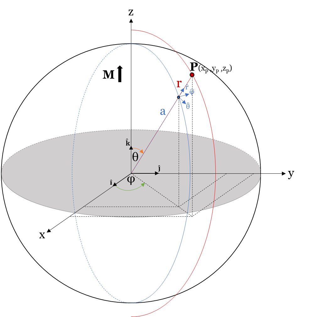
Figure 26 The magnetized sphere (blue). \(\mathbf{M}\) is in the direction of \(\mathbf{\hat{k}}\), \(r[m]\) is the distance from the center of the sphere to the observation point P, \(a [m]\) is the radius of the sphere, \(\mathbf{\hat{r}}\) is the unit vector in the direction of \(r\), \(\mathbf{\hat{\theta}}\) is the unit vector in the direction of \(\theta\), \(\theta [^{\circ}]\) is the angle between \(\mathbf{\hat{r}}\), and \(\mathbf{\hat{k}}\) increasing clockwise from \(\mathbf{\hat{k}}\)

This complete derivation is cited from [Reitz and Milford, 1960].

For the derivation of the equation of the magnetic field \(\mathbf{B}\), outside a sphere of uniformly magnetized material we revisit \(\mathbf{H}= -\nabla \psi\), eq. (14).

If situated outside of the magnetized sphere, \(\mathbf{M}=0\), therefore, equation (16) becomes \(\mathbf{B}=\mu_0\mathbf{H}\) outside the sphere.

The uniform magnetization results in \(\nabla\cdot\mathbf{H}=0\) and consequently \(\nabla^2\psi^2=0\) (Laplace’s equation). Hence, a solution of Laplace’s equation satisfying the boundary conditions is required.

If the coordinate system is chosen at the centre of the sphere and the direction of \(\mathbf{M}\) is in the polar direction (z-direction, \(\mathbf{\hat{k}}\)), the potential can be expanded in zonal harmonics. See Figure 26. Inside the material, \(\psi_I\), and outside the material, \(\psi_O\), are

(34)\[\begin{split}\begin{equation} \begin{split} & \psi_O(r,\theta) = \sum_{n=0}^{\infty} C_{1,n}r^{-1(n+1)}P_n(\theta) \\ & \psi_I(r,\theta) = \sum_{n=0}^{\infty} A_{2,n}r^{n}P_n(\theta) \end{split} \end{equation}\end{split}\]

where \(C_n\) and \(A_n\) are constants derived from boundary conditions. The boundary conditions are if \(r\rightarrow \inf\), \(\mathbf{B} \rightarrow \vec{0}\), and at \(r=a\),

(35)\[\begin{split}\begin{equation} \begin{split} & H_{O\theta} = H_{I\theta} \\ & B_{Or} = B_{Ir} \end{split} \end{equation}\end{split}\]

resulting in (for derivation \(C_n\) and \(A_n\) see [Reitz and Milford, 1960])

(36)\[\begin{split}\begin{equation} \begin{split} & \psi_O(r,\theta) =\frac{1}{3}M\frac{a^3}{r^2}\cos{\theta} \\ & \psi_I(r,\theta) =\frac{1}{3}Mr\cos{\theta} \end{split} \end{equation}\end{split}\]

using \(\mathbf{B}=\mu_0\mathbf{H}\) and \(\mathbf{H}= -\nabla \psi\), and we can define \(\mathbf{B_a}\) and \(\mathbf{B_t}\) outside a uniformally magnetized sphere as

(37)\[\begin{equation} \mathbf{B_a(r)} = \frac{\mu_{0}}{3}M\left(\frac{a^3}{r^3}\right) \left(2\mathbf{\hat{r}}\cos{\theta}+\mathbf{\hat{\theta}}\sin{\theta}\right) \end{equation}\]

and

(38)\[\begin{equation} \mathbf{B_t(r)} = B_0\mathbf{\hat{k}} + \frac{\mu_{0}}{3}M\left(\frac{a^3}{r^3}\right) \left(2\mathbf{\hat{r}}\cos{\theta}+\mathbf{\hat{\theta}}\sin{\theta}\right) \end{equation}\]

where

(39)\[\begin{split}\begin{equation} \begin{split} & \mathbf{\hat{r}} = \sin{\theta}\cos{\phi} \mathbf{\hat{i}} + \sin{\theta}\sin{\phi} \mathbf{\hat{j}} + \cos{\theta} \mathbf{\hat{k}} \\ & \mathbf{\hat{\theta}} = \cos{\theta}\cos{\phi}\mathbf{\hat{i}} + \cos{\theta}\sin{\phi}\mathbf{\hat{j}} - \sin{\theta}\mathbf{\hat{k}} \\ & \mathbf{\hat{\phi}} = -\sin{\phi}\mathbf{\hat{i}} + \cos{\phi}\mathbf{\hat{j}} \\ \end{split} \end{equation}\end{split}\]

for definitions of variables and visualization, see Figure 26.