Parameters

Replicating shapes in a discretized domain comes with inherent limitations that can potentially lead to inaccuracies in the computed values.

Following benchmarking, the next key step in the model validation process of any geodynamic model is to investigate the effect of model setup parameters and initial (boundary) conditions on the final results.

For precise and optimal anomaly computations over varied topographies, it is crucial to identify the minimum quantity of elements necessary for a accurate representation of volcanic terrain, and determining the minimal domain size to mitigate the impact of the edge effect.

This edge effect, which occurs at the boundaries of the simulated domain, emerges from the cutoff at the outer boundary of the domain, generating its own unique magnetic anomaly. Our goal is to minimize the edge effect while also managing the absolute dimensions and resolution of the domain to ensure computational efficiency and reduce the time and effort required. Furthermore, the effect of the topography of the bottom boundary of the domain will be investigated.

These parameters are determined using a domain with synthetic topography, the southern flank setup as outlined in the section flank simulations. Furthermore, the test are repeated for a zero topography setup (benchmark 2a). The experiments are conducted along a path elevated one meter above the ground, representing the minimum elevation level for most field sites with observation points approximately one meter apart. Since the lowest elevation necessitates the largest resolutions and domain size, this setup will establish the threshold.

It remains unclear whether the parameters defined through these tests can be directly correlated with the thresholds needed for calculations over topographies derived from a DEM. The real topographical variations on any volcano are anticipated to encompass larger and more intricate structures. Larger structures could potentially induce greater anomalies, which might extend farther, given that the magnitude of a magnetic anomaly generated by an entity is directly proportional to its physical properties (volume or weight) and is moderated by the distance, as noted in [Griffiths, 2013]. Consequently, a reevaluation of these parameters will be essential in upcoming DEM examinations.

Please note that the illustrations displayed here showcase only a fraction of the numerous tests executed to ascertain the necessary parameters and highlight significant discoveries. Furthermore, while these tests are specifically conducted for our case study on Mount Etna, most results are generally applicable. However, we still suggest exercising caution and recommend conducting repeated tests for future studies to ensure validity and accuracy in different contexts.

Resolution

The resolution experiments will initiate at a high resolution, gradually reducing the number of elements. We anticipate identifying a threshold where any further reduction would lead to incorrect values. Understanding the manifestation of these errors is instrumental in identifying them in other intricate setups, particularly when using the Digital Elevation Model (DEM).

Model setup

All these tests maintained a consistent domain size of \(50\times50\times120m\) for the synthetic topography setup. The expanded depth range is selected to minimize the interference from the bottom surface. To analyze this effect, some tests are conducted with a doubled domain depth of 240 meters, marked as “DD” configurations.

Variations in the number of elements are explored in both the x and y directions, fluctuating within a range of \([10:75]\) elements.

It is expected that adjusting the number of elements in the depth dimension would not impact the outcome. As, theoretically, all internal forces should negate each other, meaning that increasing this quantity would only extend the computation time.

The tests are repeated for the setup of a zero topography, however, the effect of resolution variations are expected to be redundant, as subdividing a flat surface into multiple surfaces yields no benefit, but rather will only increase computation time.

Nonetheless, these hypotheses are examined through experiments.

Results

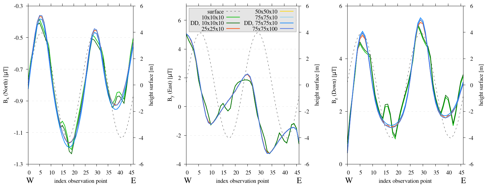
Figure 10 Three subplots depicting the components of the computed magnetic field B for the resolution experiments. The initial domain size is \(50\times50\times120m\), DD relates to extended domain depth to 240 meter, the numbers in the key relate to the amount of elements in each direction. Please note, the y-axis varies between each subplot. For an element size of \(5\times5m\), instability occurs at locations with the highest slope. An element size of \(2\times2m\) seems marginally adequate, only minor deviations occur. The amount of elements in depth does not affect results.

Figure 10 presents the findings of the resolution tests for the synthetic topography. As predicted by theory, the amount of elements in the z-direction does not affect the outcomes. For all subsequent tests, the amount of elements in the z-direction will be maintained at 10.

In the xy-directions, allocating half an element per meter proves to be marginally adequate, with only minor deviations noted for the synthetic topography results. When the resolution is reduced further, a distinctive pattern emerges; the computed values first exhibit instability at the highest slope, indicated by abrupt fluctuations in what is previously a smooth progression. Notably, an element size of \(1\times1m\) proves sufficient in these experiments.

This might initially seem contradictory to the findings of benchmark 3, which recommend increasing the element density to \(1.5\) elements per meter for observations made \(1m\) above a sphere. The contradiction is resolved by considering the sine function’s wavelength of \(25m\), which results in a decreased slope at the wave’s peak. As shown in Figure 10, the most significant errors occur at these high slopes, suggesting that tests with longer wavelengths and less spherical shapes can manage with fewer elements. This insight is crucial, especially considering that in natural environments like volcanic lava fields, topography does not typically mimic a spherical shape. Nevertheless, in synthetic topography, where such constraints do not apply, maintaining precision in future tests is essential. Therefore, future tests will aim to maintain a standard of 1.5 elements per meter in the spatial direction, wherever feasible, while staying observant of these distinctive errors.

Furthermore, Figure 10 indicates that the depth extent of the domain does not alter the observed trends stemming from insufficient resolution, but instead generates a shift in the magnetic field strength.

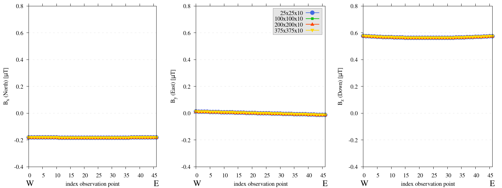
Figure 11 Three subplots depicting the components of the computed magnetic field B for the resolution experiments. The initial domain size is \(250\times250\times20m\), the numbers in the key relate to the amount of elements in each direction. The amount of elements for a flat-domain model are irrelevant.

As expected, in Figure 11 it is evident that the amount of elements for a zero topography domain are irrelevant.

Reproduce 1

Steps to reproduce the results and figures for zero topography

Please note basic setup in Installation.

1. In MTE.py, modify benchmark attribution to 2a:

   Code 56 /main/MTE.py

   benchmark = '2a'
   

2. Run first setup & move files

   Code 57 /main/MTE.py

   if benchmark == '2a':
      # General settings
      remove_zerotopo = False
      compute_analytical = False
      do_spiral_measurements = False
      do_path_measurements = False
   
      # Domain settings
      Lx, Ly, Lz = 250, 250, 20
      nelx, nely, nelz = 25, 25, 10
      Mx0, My0, Mz0 = 0, 4.085, -6.29  # Magnetization [A/m].
   
      # Plane measurement settings
      do_plane_measurements = False
      plane_nnx, plane_nny = 11, 11
      plane_x0, plane_y0, plane_z0 = -Lx / 2, -Ly / 2, 1
      plane_Lx, plane_Ly = 2 * Lx, 2 * Ly
   
      # Line measurement settings
      do_line_measurements = True
      line_nmeas = 47
      xstart, xend = 0.23 + ((Lx - 50) / 2), 49.19 + ((Ly - 50) / 2)
      ystart, yend = Ly / 2 - 0.221, Ly / 2 - 0.221
      zstart, zend = 1, 1  # 1m above surface.
   

   Code 58 /main/ (runtime: ~7 s)

   python3 -u MTE.py | tee log.txt
   

   Code 59 /main/

   mkdir -p zero_topo/restest/25_25_10 && mv log.txt *.vtu *.ascii $_
   

3. Run extra setup & move files (3)

   Code 60 /main/MTE.py # Domain settings Lx, Ly, Lz = 250, 250, 20 nelx, nely, nelz = 100, 100, 10 Mx0, My0, Mz0 = 0, 4.085, -6.29

   Code 61 /main/MTE.py # Domain settings Lx, Ly, Lz = 250, 250, 20 nelx, nely, nelz = 200, 200, 10 Mx0, My0, Mz0 = 0, 4.085, -6.29

   Code 62 /main/MTE.py # Domain settings Lx, Ly, Lz = 250, 250, 20 nelx, nely, nelz = 375, 375, 10 Mx0, My0, Mz0 = 0, 4.085, -6.29

   Code 63 /main/ (runtime: ~1 min, ~4 min, ~16 min)

   python3 -u MTE.py | tee log.txt
   

   Code 64 /main/ mkdir -p zero_topo/restest/200_200_10 && mv log.txt *.vtu *.ascii $_

   Code 65 /main/ mkdir -p zero_topo/restest/375_375_10 && mv log.txt *.vtu *.ascii $_

   Code 66 /main/ mkdir -p zero_topo/restest/100_100_10 && mv log.txt *.vtu *.ascii $_

4. Go to directory & plot to visualize

   Code 67 /main/

   cd zero_topo/
   

   Code 68 /main/zero_topo/

   gnuplot plot_script_restest.p
   

Steps to reproduce the results and figures for synthetic topography

Please note basic setup in Installation.

1. In MTE.py, modify benchmark attribution to 5, and make sure the right setup is used:

   Code 69 /main/MTE.py

   benchmark = '5'
   
   compute_vi = False  # This includes the volume integral computation by Gaussian quadrature, see
                        # documentation, possible for all setups apart from DEM (-1).
   if compute_vi:
      nqdim = 6  # Number of quadrature points, see documentation.
   
   ## ONLY BENCHMARK = -1 (DEM) & BENCHMARK = 5 (FLANKSIM) ##
   flat_bottom = True  # If True, a flat bottom is generated at the lower surface of the domain.
                       # Please see documentation, as the specific setup of this feature is different
                       # for the flank simulations and the DEM test.
   remove_zerotopo = False  # Setup run 2 times: 1st time, zero topography setup: xy coordinates
                           # of the observation points the same, but zerotopo domain and obs path
                           # shifted to average height DEM. 2nd time, "regular" run with topography.
                           # final results are 2nd run - 1 st run values. Run time can be improved,
                           # if 1st run is done with less el (and cuboid function), yet to be done.
   
   ## ONLY BENCHMARK = 5 (FLANKSIM) ##
   subbench = 'south'  # 'south', 'east', 'north', 'west', input parameters imported from flanksim
                       # have priority over any choice made here. So if this is used, make sure to
                       # comment out the import line in section below!
   global_run = False
   

2. Run first setup & move files

   Code 70 /main/MTE.py

   if benchmark == '5':
      # General settings
      do_spiral_measurements = False
      do_path_measurements = False
      compute_analytical = False
   
      # Domain settings
      Lx, Ly, Lz = 50, 50, 120
      nelx, nely, nelz = 10, 10, 10
      Mx0, My0, Mz0 = 0, 4.085, -6.29
      #Lx, Ly, Lz = 250, 250, 20
      #nelx, nely, nelz = int(Lx * 1.5), int(Ly * 1.5), 10
   
      # Synthetic topography settings
      wavelength = 25
      A = 4
      af = 6
   
      # Line measurement settings
      do_line_measurements = True
      line_nmeas = 47
      xstart, xend = 0.23 + ((Lx - 50) / 2), 49.19 + ((Ly - 50) / 2)
      ystart, yend = Ly / 2 - 0.221, Ly / 2 - 0.221
      zstart, zend = 1, 1  # 1m above surface.
   
      # Plane measurement settings
      do_plane_measurements = False
      plane_nnx, plane_nny = 30, 30
      plane_x0, plane_y0, plane_z0 = -Lx / 2, -Ly / 2, 1
      plane_Lx, plane_Ly = 2 * Lx, 2 * Ly
   
      #from flanksim import *
   

   Code 71 /main/ (runtime: ~6 s)

   python3 -u MTE.py | tee log.txt
   

   Code 72 /main/

   mkdir -p flanksim_parameters/south/restest/10_10_10 && mv log.txt *.vtu *.ascii $_
   

3. Run extra setups & move files (6)

   Code 73 /main/MTE.py # Domain settings Lx, Ly, Lz = 50, 50, 240 nelx, nely, nelz = 10, 10, 10 Mx0, My0, Mz0 = 0, 4.085, -6.29

   Code 74 /main/MTE.py # Domain settings Lx, Ly, Lz = 50, 50, 120 nelx, nely, nelz = 25, 25, 10 Mx0, My0, Mz0 = 0, 4.085, -6.29

   Code 75 /main/MTE.py # Domain settings Lx, Ly, Lz = 50, 50, 120 nelx, nely, nelz = 50, 50, 10 Mx0, My0, Mz0 = 0, 4.085, -6.29

   Code 76 /main/MTE.py # Domain settings Lx, Ly, Lz = 50, 50, 120 nelx, nely, nelz = 75, 75, 10 Mx0, My0, Mz0 = 0, 4.085, -6.29

   Code 77 /main/MTE.py # Domain settings Lx, Ly, Lz = 50, 50, 120 nelx, nely, nelz = 75, 75, 100 Mx0, My0, Mz0 = 0, 4.085, -6.29

   Code 78 /main/MTE.py # Domain settings Lx, Ly, Lz = 50, 50, 240 nelx, nely, nelz = 75, 75, 10 Mx0, My0, Mz0 = 0, 4.085, -6.29

   Code 79 /main/ (runtime: ~6 s, ~12 s, ~35 s, ~1 min, ~12 min, ~1 min)

   python3 -u MTE.py | tee log.txt
   

   Code 80 /main/ mkdir -p flanksim_parameters/south/restest/10_10_10_DD && mv log.txt *.vtu *.ascii $_

   Code 81 /main/ mkdir -p flanksim_parameters/south/restest/25_25_10 && mv log.txt *.vtu *.ascii $_

   Code 82 /main/ mkdir -p flanksim_parameters/south/restest/50_50_10 && mv log.txt *.vtu *.ascii $_

   Code 83 /main/ mkdir -p flanksim_parameters/south/restest/75_75_10 && mv log.txt *.vtu *.ascii $_

   Code 84 /main/ mkdir -p flanksim_parameters/south/restest/75_75_100 && mv log.txt *.vtu *.ascii $_

   Code 85 /main/ mkdir -p flanksim_parameters/south/restest/75_75_10_DD && mv log.txt *.vtu *.ascii $_

4. Go to directory & plot to visualize

   Code 86 /main/

   cd flanksim_parameters/
   

   Code 87 /main/flanksim_parameters/

   gnuplot plot_script_restest.p
   

Size

The size experiments will commence with a more compact domain and progressively expand it until the computed magnetic field at a point above the domain center stabilizes. The outcomes of changes in both the depth extent (z-direction) and spatial extent (xy-direction) will be analyzed.

However, upon adapting domain depth, a complication arises: the exact nature of the magnetization in the underlying flows and deeper is unknown. Nonetheless, a uniform magnetization is continuously assumed. This assumption now expands deeper, eventually stretching to the full pile of volcanic flows of Mount Etna. To validate this assumption for our case study, we refer to the geomagnetic history of Mount Etna. The last reversal of Earth’s magnetic field is dated around \(\sim795\) ka ago [Singer et al., 2019] and the first volcanic activity of Mount Etna is dated around \(\sim500\) ka ago [Branca et al., 2008].

Therefore, no reversals are anticipated within the accumulated layers, allowing us to extend the depth for experimental purposes without restrictions. Nonetheless, as the directly underlying flow is deemed to exert the most substantial influence, expanding the depth beyond a singular flow might be redundant. The thickness of the flows underneath the field sites mentioned in [Meyer and de Groot, 2024] fluctuate between 5-15 meter [Andronico et al., 2005, Murray and Stevens, 2000].

Model setup

Consequently, our tests explore domain depth ranging from \([5:1800]\) meter, and a spatial extent from \([50:1000]\) meter. The experiments will be done maintaining element resolution consistent with the previously established threshold at observation points along a path one meter above the surface.

Results and analysis

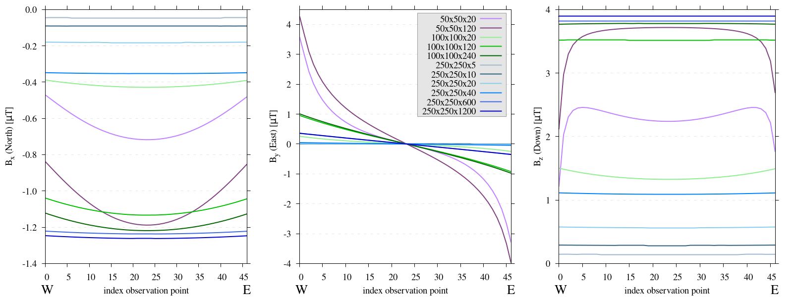
Figure 12 Three subplots depicting the components of the computed magnetic field B for the size experiments. The numbers in the key relate to the length of each side of the domain (Lx_Ly_Lz). Please note, the y-axis varies between each subplot. For domains with spatial extent below \(250\times250m\) an edge effect is observed. Additionally, a relationship between extent of the domain and magnitude of the anomaly is evident, this will be further explored in the next Figure.

In the investigations presented in Figure 12, spatial extents below \(250\times250m\) prominently display edge effects. This is particularly evident for the \(B_y\) component, which should ideally measure zero in the absence of topography or declination in magnetization. A uniform value across the observation path indicates the absence of edge effects, whereas variable values correlate with proximity to the domain edge.

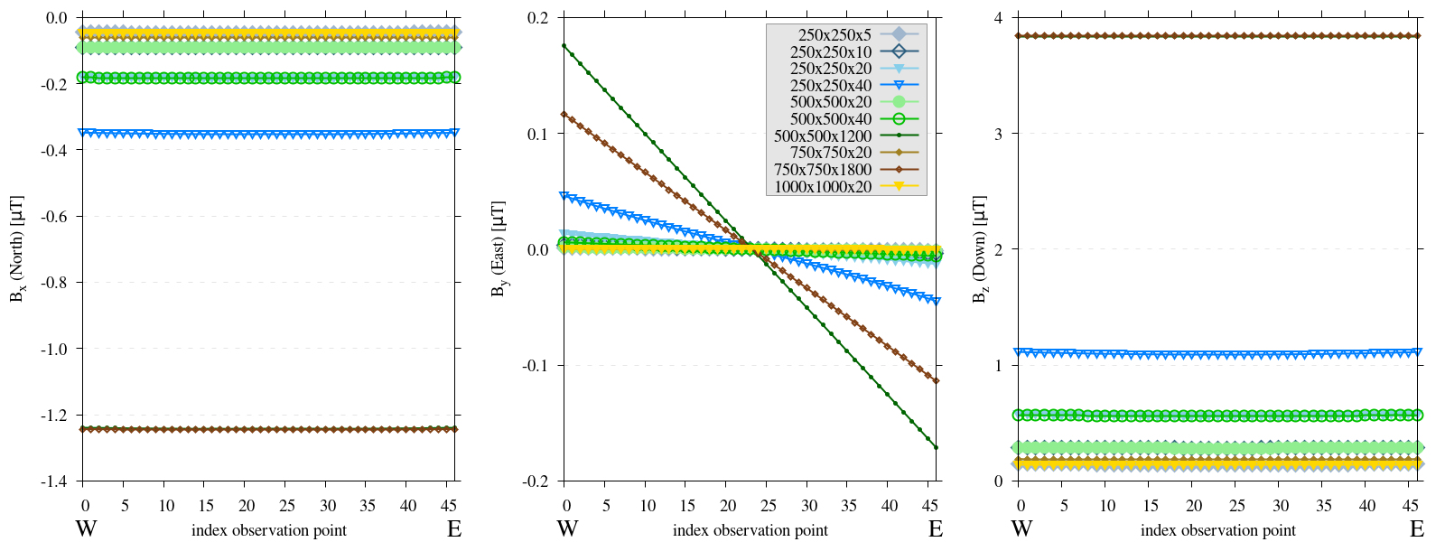
Figure 13 Three subplots depicting the components of the computed magnetic field B for the size experiments. The numbers in the key relate to the length of each side of the domain (Lx_Ly_Lz). Please note, the y-axis varies between each subplot. The relationship between extent of the domain and magnitude of the anomaly is prominently displayed, increasing depth enhances components \(B_x\) and \(B_z\) proportionally, while increasing spatial extent leads to a similarly proportional reduction of these components. Furthermore, increasing depth emphasizes the edge effect displayed.

Our data reveals a nuanced relationship between the depth and spatial extent of the domain and the anomaly’s intensity, as evident in both Figure 12 and Figure 13. Notably, for components \(B_x\) and \(B_z\), magnitude increases with depth in a non-linear fashion. An initial increase in depth (\(10\) to \(600\) meter) yields a significant change in component values, but a subsequent increase from \(600\) to \(1200\) meter sees marginal differences. This relationship also depends on spatial extent. For instance, \(500\times500\times40\) and \(250\times250\times20\) meter configurations produce identical \(B_x\) and \(B_z\) values. Observations unveil three distinct patterns, see Figure 13:

1. Identical values arise when both depth and spatial extent increase equivalently (e.g., \(250\times250\times20\) and \(500\times500\times40\) meters).

2. Increasing spatial extent alone reduces the magnitude proportionally (e.g., \(250\times250\times20\) and \(500\times500\times20\) meters).

3. Increasing depth alone enhances the magnitude proportionally (e.g., \(500\times500\times20\) and \(500\times500\times40\) meters).

It is important to highlight that the inclination values are consistent across different setups, given that the modulating factor for both \(B_x\) and \(B_z\) remains identical.

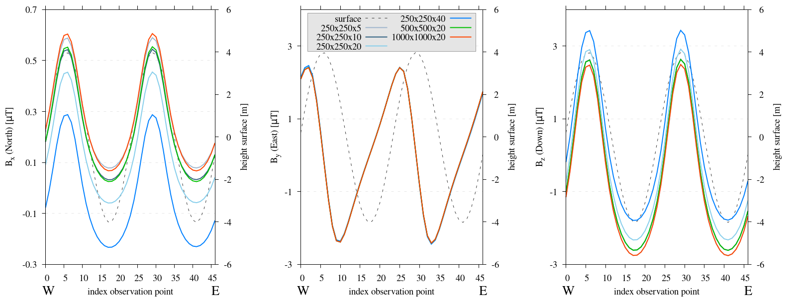
Figure 14 Three subplots depicting the components of the computed magnetic field B for the depth experiments. Size and depth of the domain are varied, the resolution and relative location (centered in the domain) of the observation path are constant. Components are rotated to align with Pmag coordinate system. The numbers in the key relate to the length of each side of the domain (Lx_Ly_Lz). Please note, the y-axis varies between each subplot. Similar trends as before are visible, spatial and depth extent proportionally influence the magnitude of the \(B_z\) and \(B_x\) components. However, for domains with a smaller depth extent, these differences are minimal compared to the anomalies produced by the topography.

Figure 14 display the outcomes from testing the domain size constraints on a simulation with topography, and displays similar trends with respect to required spatial extent and relationship between spatial dimension and magnitude of components. Extending the depth and spatial extent has a proportional impact on the magnitude of the \(B_z\) and \(B_x\) components.

Reproduce

Steps to reproduce the results and figures for zero topography

Please note basic setup in Installation.

1. In MTE.py, modify benchmark attribution to 2a:

   Code 88 /main/MTE.py

   benchmark = '2a'
   

2. Run first setup & move files

   Code 89 /main/MTE.py

   if benchmark == '2a':
      # General settings
      remove_zerotopo = False
      compute_analytical = False
      do_spiral_measurements = False
      do_path_measurements = False
   
      # Domain settings
      Lx, Ly, Lz = 50, 50, 20
      nelx, nely, nelz = int(Lx), int(Ly), 10
      Mx0, My0, Mz0 = 0, 4.085, -6.29  # Magnetization [A/m].
   
      # Plane measurement settings
      do_plane_measurements = False
      plane_nnx, plane_nny = 11, 11
      plane_x0, plane_y0, plane_z0 = -Lx / 2, -Ly / 2, 1
      plane_Lx, plane_Ly = 2 * Lx, 2 * Ly
   
      # Line measurement settings
      do_line_measurements = True
      line_nmeas = 47
      xstart, xend = 0.23 + ((Lx - 50) / 2), 49.19 + ((Ly - 50) / 2)
      ystart, yend = Ly / 2 - 0.221, Ly / 2 - 0.221
      zstart, zend = 1, 1  # 1m above surface.
   

   Code 90 /main/ (runtime: ~20 s)

   python3 -u MTE.py | tee log.txt
   

   Code 91 /main/

   mkdir -p zero_topo/50_50_20 && mv log.txt *.vtu *.ascii $_
   

3. Run extra setups & move files (16)

   Code 92 /main/MTE.py # Domain settings Lx, Ly, Lz = 50, 50, 120 nelx, nely, nelz = int(Lx), int(Ly), 10 Mx0, My0, Mz0 = 0, 4.085, -6.29

   Code 93 /main/MTE.py # Domain settings Lx, Ly, Lz = 100, 100, 20 nelx, nely, nelz = int(Lx), int(Ly), 10 Mx0, My0, Mz0 = 0, 4.085, -6.29

   Code 94 /main/MTE.py # Domain settings Lx, Ly, Lz = 100, 100, 120 nelx, nely, nelz = int(Lx), int(Ly), 10 Mx0, My0, Mz0 = 0, 4.085, -6.29

   Code 95 /main/MTE.py # Domain settings Lx, Ly, Lz = 100, 100, 240 nelx, nely, nelz = int(Lx), int(Ly), 10 Mx0, My0, Mz0 = 0, 4.085, -6.29

   Code 96 /main/MTE.py # Domain settings Lx, Ly, Lz = 250, 250, 5 nelx, nely, nelz = int(Lx), int(Ly), 10 Mx0, My0, Mz0 = 0, 4.085, -6.29

   Code 97 /main/MTE.py # Domain settings Lx, Ly, Lz = 250, 250, 10 nelx, nely, nelz = int(Lx), int(Ly), 10 Mx0, My0, Mz0 = 0, 4.085, -6.29

   Code 98 /main/MTE.py # Domain settings Lx, Ly, Lz = 250, 250, 20 nelx, nely, nelz = int(Lx), int(Ly), 10 Mx0, My0, Mz0 = 0, 4.085, -6.29

   Code 99 /main/MTE.py # Domain settings Lx, Ly, Lz = 250, 250, 40 nelx, nely, nelz = int(Lx), int(Ly), 10 Mx0, My0, Mz0 = 0, 4.085, -6.29

   Code 100 /main/MTE.py # Domain settings Lx, Ly, Lz = 250, 250, 600 nelx, nely, nelz = int(Lx), int(Ly), 10 Mx0, My0, Mz0 = 0, 4.085, -6.29

   Code 101 /main/MTE.py # Domain settings Lx, Ly, Lz = 250, 250, 1200 nelx, nely, nelz = int(Lx), int(Ly), 10 Mx0, My0, Mz0 = 0, 4.085, -6.29

   Code 102 /main/MTE.py # Domain settings Lx, Ly, Lz = 500, 500, 20 nelx, nely, nelz = int(Lx), int(Ly), 10 Mx0, My0, Mz0 = 0, 4.085, -6.29

   Code 103 /main/MTE.py # Domain settings Lx, Ly, Lz = 500, 500, 40 nelx, nely, nelz = int(Lx), int(Ly), 10 Mx0, My0, Mz0 = 0, 4.085, -6.29

   Code 104 /main/MTE.py # Domain settings Lx, Ly, Lz = 500, 500, 1200 nelx, nely, nelz = int(Lx), int(Ly), 10 Mx0, My0, Mz0 = 0, 4.085, -6.29

   Code 105 /main/MTE.py # Domain settings Lx, Ly, Lz = 750, 750, 20 nelx, nely, nelz = int(Lx), int(Ly), 10 Mx0, My0, Mz0 = 0, 4.085, -6.29

   Code 106 /main/MTE.py # Domain settings Lx, Ly, Lz = 750, 750, 1800 nelx, nely, nelz = int(Lx), int(Ly), 10 Mx0, My0, Mz0 = 0, 4.085, -6.29

   Code 107 /main/MTE.py # Domain settings Lx, Ly, Lz = 1000, 1000, 20 nelx, nely, nelz = int(Lx), int(Ly), 10 Mx0, My0, Mz0 = 0, 4.085, -6.29

   Code 108 /main/ (runtime: ~20 s, ~1 min, ~1 min, ~1 min, ~7 min, ~7 min, ~7 min, ~7 min, ~7 min, ~7 min, ~30 min, ~30 min, ~30 min, ~1 hr, ~1 hr, ~2 hr)

   python3 -u MTE.py | tee log.txt
   

   Code 109 /main/ mkdir -p zero_topo/50_50_120 && mv log.txt *.vtu *.ascii $_

   Code 110 /main/ mkdir -p zero_topo/100_100_20 && mv log.txt *.vtu *.ascii $_

   Code 111 /main/ mkdir -p zero_topo/100_100_120 && mv log.txt *.vtu *.ascii $_

   Code 112 /main/ mkdir -p zero_topo/100_100_240 && mv log.txt *.vtu *.ascii $_

   Code 113 /main/ mkdir -p zero_topo/250_250_5 && mv log.txt *.vtu *.ascii $_

   Code 114 /main/ mkdir -p zero_topo/250_250_10 && mv log.txt *.vtu *.ascii $_

   Code 115 /main/ mkdir -p zero_topo/250_250_20 && mv log.txt *.vtu *.ascii $_

   Code 116 /main/ mkdir -p zero_topo/250_250_40 && mv log.txt *.vtu *.ascii $_

   Code 117 /main/ mkdir -p zero_topo/250_250_600 && mv log.txt *.vtu *.ascii $_

   Code 118 /main/ mkdir -p zero_topo/250_250_1200 && mv log.txt *.vtu *.ascii $_

   Code 119 /main/ mkdir -p zero_topo/500_500_20 && mv log.txt *.vtu *.ascii $_

   Code 120 /main/ mkdir -p zero_topo/500_500_40 && mv log.txt *.vtu *.ascii $_

   Code 121 /main/ mkdir -p zero_topo/500_500_1200 && mv log.txt *.vtu *.ascii $_

   Code 122 /main/ mkdir -p zero_topo/500_500_1200 && mv log.txt *.vtu *.ascii $_

   Code 123 /main/ mkdir -p zero_topo/750_750_1800 && mv log.txt *.vtu *.ascii $_

   Code 124 /main/ mkdir -p zero_topo/1000_1000_20 && mv log.txt *.vtu *.ascii $_

4. Go to directory & plot to visualize

   Code 125 /main/

   cd zero_topo/
   

   Code 126 /main/zero_topo/

   gnuplot plot_script_extest.p
   

Steps to reproduce the results and figures for synthetic topography

Please note basic setup in Installation.

1. In MTE.py, modify benchmark attribution to 5, and make sure the right setup is used:

   Code 127 /main/MTE.py

   benchmark = '5'
   
   compute_vi = False  # This includes the volume integral computation by Gaussian quadrature, see
                        # documentation, possible for all setups apart from DEM (-1).
   if compute_vi:
      nqdim = 6  # Number of quadrature points, see documentation.
   
   ## ONLY BENCHMARK = -1 (DEM) & BENCHMARK = 5 (FLANKSIM) ##
   flat_bottom = True  # If True, a flat bottom is generated at the lower surface of the domain.
                       # Please see documentation, as the specific setup of this feature is different
                       # for the flank simulations and the DEM test.
   remove_zerotopo = False  # Setup run 2 times: 1st time, zero topography setup: xy coordinates
                           # of the observation points the same, but zerotopo domain and obs path
                           # shifted to average height DEM. 2nd time, "regular" run with topography.
                           # final results are 2nd run - 1 st run values. Run time can be improved,
                           # if 1st run is done with less el (and cuboid function), yet to be done.
   
   ## ONLY BENCHMARK = 5 (FLANKSIM) ##
   subbench = 'south'  # 'south', 'east', 'north', 'west', input parameters imported from flanksim
              # have priority over any choice made here. So if this is used, make sure to
              # comment out the import line in section below!
   global_run = False
   

2. Run first setup & move files

   Code 128 /main/MTE.py

   if benchmark == '5':
      # General settings
      do_spiral_measurements = False
      do_path_measurements = False
      compute_analytical = False
   
      # Domain settings
      Lx, Ly, Lz = 250, 250, 5
      nelx, nely, nelz = int(Lx * 1.5), int(Ly * 1.5), 10
      Mx0, My0, Mz0 = 0, 4.085, -6.29
      #Lx, Ly, Lz = 50, 50, 120
      #nelx, nely, nelz = 10, 10, 10
   
      # Synthetic topography settings
      wavelength = 25
      A = 4
      af = 6
   
      # Line measurement settings
      do_line_measurements = True
      line_nmeas = 47
      xstart, xend = 0.23 + ((Lx - 50) / 2), 49.19 + ((Ly - 50) / 2)
      ystart, yend = Ly / 2 - 0.221, Ly / 2 - 0.221
      zstart, zend = 1, 1  # 1m above surface.
   
      # Plane measurement settings
      do_plane_measurements = False
      plane_nnx, plane_nny = 30, 30
      plane_x0, plane_y0, plane_z0 = -Lx / 2, -Ly / 2, 1
      plane_Lx, plane_Ly = 2 * Lx, 2 * Ly
   

   Code 129 /main/ (runtime: ~30 min)

   python3 -u MTE.py | tee log.txt
   

   Code 130 /main/

   mkdir -p flanksim_parameters/south/extest/250_250_5 && mv log.txt *.vtu *.ascii $_
   

3. Run extra setups & move files (5)

   Code 131 /main/MTE.py # Domain settings Lx, Ly, Lz = 250, 250, 10

   Code 132 /main/MTE.py # Domain settings Lx, Ly, Lz = 250, 250, 20

   Code 133 /main/MTE.py # Domain settings Lx, Ly, Lz = 250, 250, 40

   Code 134 /main/MTE.py # Domain settings Lx, Ly, Lz = 500, 500, 20

   Code 135 /main/MTE.py # Domain settings Lx, Ly, Lz = 1000, 1000, 20

   Code 136 /main/ (runtime: ~30 min, ~30 min, ~30 min, ~2 hr, ~8 hr)

   python3 -u MTE.py | tee log.txt
   

   Code 137 /main/ mkdir -p flanksim_parameters/south/extest/250_250_10 && mv log.txt *.vtu *.ascii $_

   Code 138 /main/ mkdir -p flanksim_parameters/south/extest/250_250_20 && mv log.txt *.vtu *.ascii $_

   Code 139 /main/ mkdir -p flanksim_parameters/south/extest/250_250_40 && mv log.txt *.vtu *.ascii $_

   Code 140 /main/ mkdir -p flanksim_parameters/south/extest/500_500_20 && mv log.txt *.vtu *.ascii $_

   Code 141 /main/ mkdir -p flanksim_parameters/south/extest/1000_1000_20 && mv log.txt *.vtu *.ascii $_

4. Go to directory & plot to visualize

   Code 142 /main/

   cd flanksim_parameters/
   

   Code 143 /main/flanksim_parameters/

   gnuplot plot_script_extest.p
   

Verification

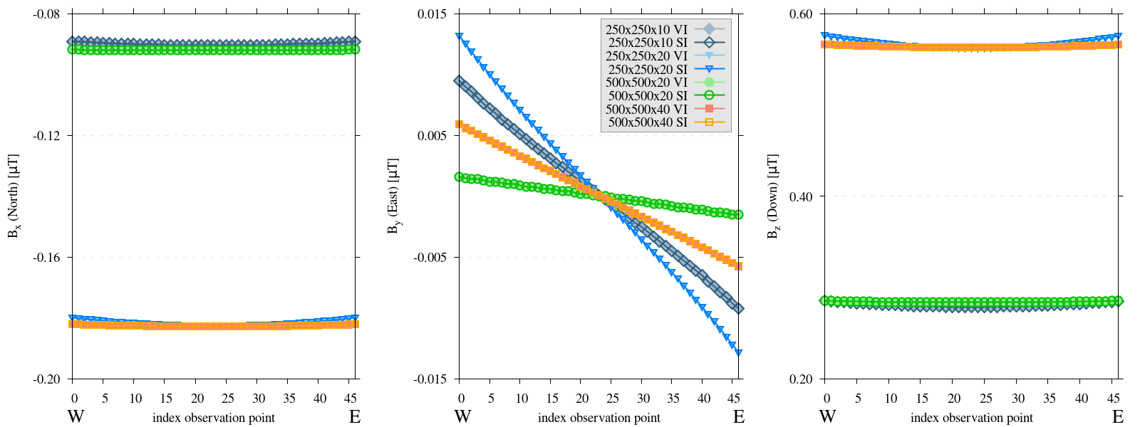
Figure 15 Three subplots depicting the components of the computed magnetic field B for flat-terrain experiments. The spatial extent of the domain is varied, while adhering the threshold resolution. The numbers in the key relate to the length of each side of the domain (Lx_Ly_Lz). Results marked ‘VI’ were derived using the volume integral method, whereas those labeled ‘SI’ were obtained via the surface integral method. Please note, the y-axis varies between each subplot. Consistently, both methods generate identical results, with the previously described trends observable in both cases.

3D Gauss-Legendre quadrature rules are adopted to numerically determine the volume integral (see equation (19)). This methodology served as a reference due to the absence of published benchmarks. Remarkably, our essentially analytical solutions align closely with the numerical approximations, see Figure 15, which suggests that the observed trends are not computational but more theoretical in nature.

Reproduce

Steps to reproduce the results and figures for zero topography

Please note basic setup in Installation.

1. In MTE.py, modify benchmark attribution to 2a:

   Code 144 /main/MTE.py

   benchmark = '2a'
   
   compute_vi = True  # This includes the volume integral computation by Gaussian quadrature, see
                        # documentation, possible for all setups apart from DEM (-1).
   if compute_vi:
      nqdim = 6  # Number of quadrature points, see documentation.
   

2. Run first setup & move files

   Code 145 /main/MTE.py

   if benchmark == '2a':
      # General settings
      remove_zerotopo = False
      compute_analytical = False
      do_spiral_measurements = False
      do_path_measurements = False
   
      # Domain settings
      Lx, Ly, Lz = 250, 250, 10
      nelx, nely, nelz = int(Lx), int(Ly), 10
      Mx0, My0, Mz0 = 0, 4.085, -6.29  # Magnetization [A/m].
   
      # Plane measurement settings
      do_plane_measurements = False
      plane_nnx, plane_nny = 11, 11
      plane_x0, plane_y0, plane_z0 = -Lx / 2, -Ly / 2, 1
      plane_Lx, plane_Ly = 2 * Lx, 2 * Ly
   
      # Line measurement settings
      do_line_measurements = True
      line_nmeas = 47
      xstart, xend = 0.23 + ((Lx - 50) / 2), 49.19 + ((Ly - 50) / 2)
      ystart, yend = Ly / 2 - 0.221, Ly / 2 - 0.221
      zstart, zend = 1, 1  # 1m above surface.
   

   Code 146 /main/ (runtime: ~2.5 hr)

   python3 -u MTE.py | tee log.txt
   

   Code 147 /main/

   mkdir -p zero_topo/250_250_10_wvi && mv log.txt *.vtu *.ascii $_
   

3. Run extra setups & move files (3)

   Code 148 /main/MTE.py # Domain settings Lx, Ly, Lz = 250, 250, 20 nelx, nely, nelz = int(Lx), int(Ly), 10 Mx0, My0, Mz0 = 0, 4.085, -6.29

   Code 149 /main/MTE.py # Domain settings Lx, Ly, Lz = 500, 500, 20 nelx, nely, nelz = int(Lx), int(Ly), 10 Mx0, My0, Mz0 = 0, 4.085, -6.29

   Code 150 /main/MTE.py # Domain settings Lx, Ly, Lz = 500, 500, 40 nelx, nely, nelz = int(Lx), int(Ly), 10 Mx0, My0, Mz0 = 0, 4.085, -6.29

   Code 151 /main/ (runtime: ~2.5 hr, ~10 hr, ~10 hr)

   python3 -u MTE.py | tee log.txt
   

   Code 152 /main/ mkdir -p zero_topo/250_250_20_wvi && mv log.txt *.vtu *.ascii $_

   Code 153 /main/ mkdir -p zero_topo/500_500_20_wvi && mv log.txt *.vtu *.ascii $_

   Code 154 /main/ mkdir -p zero_topo/500_500_40_wvi && mv log.txt *.vtu *.ascii $_

4. Go to directory & plot to visualize

   Code 155 /main/

   cd zero_topo/
   

   Code 156 /main/zero_topo/

   gnuplot plot_script_visi.p
   

Challenges in Setup Optimization

Determining the optimal setup for the size of the domain now poses challenges. While increasing domain size might intuitively stabilize computed values, Figure 14, Figure 12 and Figure 13 contradict this presumption. While consistent depth expansion appears to eventually plateau the results, increasing depth continues to influence the magnitudes of the \(B_x\) and \(B_z\) components, as illustrated in various depth configurations with a spatial layout of \(250\times250m\) in Figure 12. Moreover, when comparing deeper configurations like \(500\times500\times1800\) with \(500\times500\times20\) meters in Figure 12, a pronounced amplification of edge effects for the \(B_y\) component is evident. This observation aligns with recommendations from the foundational study by [Bott, 1963], suggesting that optimal results emerge when the depth is substantially less than the areal extent.

Nevertheless, this observation does not offer clarity in distinguishing between configurations of shallower depths but varied spatial dimensions, such as \(250\times250\times10\), \(250\times250\times20\), \(500\times500\times20\), \(500\times500\times40\) meters. Still, by examining Figure 14, it becomes apparent that magnitude differences for these setups are minimal when juxtaposed with anomalies caused by topography.

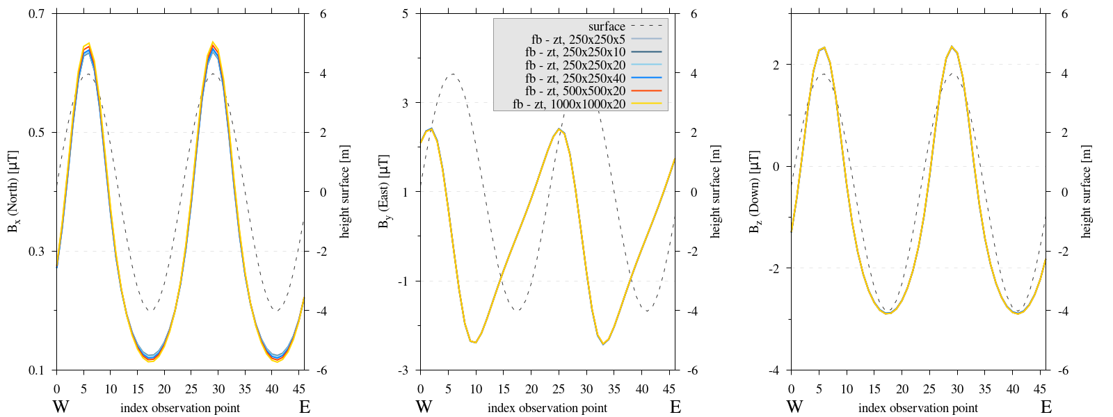
Figure 16 Three subplots depicting the components of the computed magnetic field B for the depth experiments. The numbers in the key relate to the length of each side of the domain (Lx_Ly_Lz). Please note, the y-axis varies between each subplot. Adjusting the computed values with a zero topography run removes most domain related variations, irrelevant of size and depth.

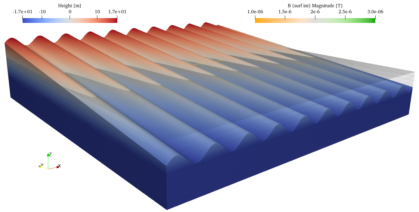
Figure 17 Visualization of Southern flank and flat-terrain model setup. The flat-terrain setup is set to a lower opacity, to show the intersection between the two domains. The observation points for both setups are at the same xy-coordinates, only the z-coordinate differs. Furthermore, the thickness of the flat-terrain domain is equal to the depth of the topography setup underneath the observation path.

Furthermore, by adjusting the computed values at the observation points for the topographic model with computed values for a flat-terrain model with matching dimensions, the discrepancies nearly converge into a single solution, as illustrated in Figure 16. The residual minor fluctuations in the \(B_x\) components across various domain sizes may stem from the incline of the topographic model. In consideration that this method essentially involves subtracting a rectangular prism from the simulation of the southern slope, which ascends northward, see Figure 17. It is important to note that the flat-terrain domain, chosen for subtraction, is configured with a vertical span equal to the depth of the domain underneath the observation path, aligning with elements that most significantly affect the final calculations.

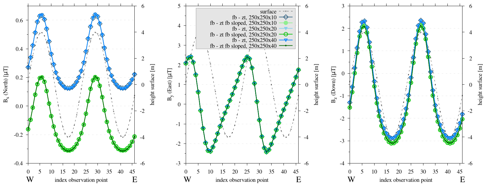
Figure 18 Three subplots depicting the components of the computed magnetic field B for the depth experiments. The numbers in the key relate to the length of each side of the domain (Lx_Ly_Lz). Please note, the y-axis varies between each subplot. Subtracting a sloped zero-topography instead of a regular flat zero-topography domain results in the \(B_x\) components to fully match. However, it is evident that the effect of the slope is also removed, as the results are approximately \(0.5 \mu T\) lower than in previous tests.

As evidenced in Figure 18, removing a sloped “flat”-terrain model from the calculations causes the solutions for all domain sizes to merge into a single solution, which also, unfortunately, removes the slope’s effect from the output. This removal is counterproductive since lava flows frequently are deposited on volcanic slopes.

Therefore, and again highlighting that these anomalies are small compared to the topographic anomalies being studies, it is recommended for more complex domain configurations to remove flat-terrain model’s results to cancel out any effects of the domain size on the findings. Future investigation should also meticulously evaluate the role of both the depth and the spatial extent of the domain.

This study’s focal point is the influence of topography on magnetic field readings above a flow, thus, this subtraction technique is adequate for alleviating complications linked to domain size and the magnitude of the resultant anomaly. A key takeaway is that maintaining a spatial size above or equal to 250x250 meter, where the depth is considerably less than the spatial dimension, is crucial.

Reproduce

Steps to reproduce the results and figures for synthetic topography

Please note basic setup in Installation.

1. In MTE.py, modify benchmark attribution to 5, and make sure the right setup is used:

   Code 157 /main/MTE.py

   benchmark = '5'
   
   compute_vi = False  # This includes the volume integral computation by Gaussian quadrature, see
                        # documentation, possible for all setups apart from DEM (-1).
   if compute_vi:
      nqdim = 6  # Number of quadrature points, see documentation.
   
   ## ONLY BENCHMARK = -1 (DEM) & BENCHMARK = 5 (FLANKSIM) ##
   flat_bottom = True  # If True, a flat bottom is generated at the lower surface of the domain.
                       # Please see documentation, as the specific setup of this feature is different
                       # for the flank simulations and the DEM test.
   remove_zerotopo = True  # Setup run 2 times: 1st time, zero topography setup: xy coordinates
                           # of the observation points the same, but zerotopo domain and obs path
                           # shifted to average height DEM. 2nd time, "regular" run with topography.
                           # final results are 2nd run - 1 st run values. Run time can be improved,
                           # if 1st run is done with less el (and cuboid function), yet to be done.
   
   ## ONLY BENCHMARK = 5 (FLANKSIM) ##
   subbench = 'south'  # 'south', 'east', 'north', 'west', input parameters imported from flanksim
              # have priority over any choice made here. So if this is used, make sure to
              # comment out the import line in section below!
   global_run = False
   

2. Run first setup & move files

   Code 158 /main/MTE.py

   if benchmark == '5':
      # General settings
      do_spiral_measurements = False
      do_path_measurements = False
      compute_analytical = False
   
      # Domain settings
      Lx, Ly, Lz = 250, 250, 5
      nelx, nely, nelz = int(Lx * 1.5), int(Ly * 1.5), 10
      Mx0, My0, Mz0 = 0, 4.085, -6.29
      #Lx, Ly, Lz = 50, 50, 120
      #nelx, nely, nelz = 10, 10, 10
   
      # Synthetic topography settings
      wavelength = 25
      A = 4
      af = 6
   
      # Line measurement settings
      do_line_measurements = True
      line_nmeas = 47
      xstart, xend = 0.23 + ((Lx - 50) / 2), 49.19 + ((Ly - 50) / 2)
      ystart, yend = Ly / 2 - 0.221, Ly / 2 - 0.221
      zstart, zend = 1, 1  # 1m above surface.
   
      # Plane measurement settings
      do_plane_measurements = False
      plane_nnx, plane_nny = 30, 30
      plane_x0, plane_y0, plane_z0 = -Lx / 2, -Ly / 2, 1
      plane_Lx, plane_Ly = 2 * Lx, 2 * Ly
   

   Code 159 /main/

   python3 -u MTE.py | tee log.txt
   

   Code 160 /main/

   mkdir -p flanksim_parameters/south/ztr/250_250_5 && mv log.txt *.vtu *.ascii $_
   

3. Run extra setups & move files (5)

   Code 161 /main/MTE.py # Domain settings Lx, Ly, Lz = 250, 250, 10

   Code 162 /main/MTE.py # Domain settings Lx, Ly, Lz = 250, 250, 20

   Code 163 /main/MTE.py # Domain settings Lx, Ly, Lz = 250, 250, 40

   Code 164 /main/MTE.py # Domain settings Lx, Ly, Lz = 500, 500, 20

   Code 165 /main/MTE.py # Domain settings Lx, Ly, Lz = 1000, 1000, 20

   Code 166 /main/ (runtime: ~1 hr, ~1 hr, ~1 hr, ~4 hr, ~16 hr)

   python3 -u MTE.py | tee log.txt
   

   Code 167 /main/ mkdir -p flanksim_parameters/south/ztr/250_250_10 && mv log.txt *.vtu *.ascii $_

   Code 168 /main/ mkdir -p flanksim_parameters/south/ztr/250_250_20 && mv log.txt *.vtu *.ascii $_

   Code 169 /main/ mkdir -p flanksim_parameters/south/ztr/250_250_40 && mv log.txt *.vtu *.ascii $_

   Code 170 /main/ mkdir -p flanksim_parameters/south/ztr/500_500_20 && mv log.txt *.vtu *.ascii $_

   Code 171 /main/ mkdir -p flanksim_parameters/south/ztr/1000_1000_20 && mv log.txt *.vtu *.ascii $_

4. Run three sloped zero topography setups & move files

   Code 172 /main/MTE.py

   benchmark = '5'
   
   compute_vi = False  # This includes the volume integral computation by Gaussian quadrature, see
                        # documentation, possible for all setups apart from DEM (-1).
   if compute_vi:
      nqdim = 6  # Number of quadrature points, see documentation.
   
   ## ONLY BENCHMARK = -1 (DEM) & BENCHMARK = 5 (FLANKSIM) ##
   flat_bottom = True  # If True, a flat bottom is generated at the lower surface of the domain.
                       # Please see documentation, as the specific setup of this feature is different
                       # for the flank simulations and the DEM test.
   remove_zerotopo = False  # Setup run 2 times: 1st time, zero topography setup: xy coordinates
                           # of the observation points the same, but zerotopo domain and obs path
                           # shifted to average height DEM. 2nd time, "regular" run with topography.
                           # final results are 2nd run - 1 st run values. Run time can be improved,
                           # if 1st run is done with less el (and cuboid function), yet to be done.
   
   ## ONLY BENCHMARK = 5 (FLANKSIM) ##
   subbench = 'south'  # 'south', 'east', 'north', 'west', input parameters imported from flanksim
              # have priority over any choice made here. So if this is used, make sure to
              # comment out the import line in section below!
   global_run = False
   

   Code 173 /main/MTE.py # Domain settings Lx, Ly, Lz = 250, 250, 10 nelx, nely, nelz = int(Lx * 1.5), int(Ly * 1.5), 10 Mx0, My0, Mz0 = 0, 4.085, -6.29 #Lx, Ly, Lz = 50, 50, 120 #nelx, nely, nelz = 10, 10, 10 # Synthetic topography settings wavelength = 0 A = 0 af = 6

   Code 174 /main/MTE.py # Domain settings Lx, Ly, Lz = 250, 250, 20 nelx, nely, nelz = int(Lx * 1.5), int(Ly * 1.5), 10 Mx0, My0, Mz0 = 0, 4.085, -6.29 #Lx, Ly, Lz = 50, 50, 120 #nelx, nely, nelz = 10, 10, 10 # Synthetic topography settings wavelength = 0 A = 0 af = 6

   Code 175 /main/MTE.py # Domain settings Lx, Ly, Lz = 250, 250, 40 nelx, nely, nelz = int(Lx * 1.5), int(Ly * 1.5), 10 Mx0, My0, Mz0 = 0, 4.085, -6.29 #Lx, Ly, Lz = 50, 50, 120 #nelx, nely, nelz = 10, 10, 10 # Synthetic topography settings wavelength = 0 A = 0 af = 6

   Code 176 /main/ (runtime: ~30 min, ~30 min, ~30 min)

   python3 -u MTE.py | tee log.txt
   

   Code 177 /main/ mkdir -p flanksim_parameters/south/ztr/250_250_10_ss && mv log.txt *.vtu *.ascii $_

   Code 178 /main/ mkdir -p flanksim_parameters/south/ztr/250_250_20_ss && mv log.txt *.vtu *.ascii $_

   Code 179 /main/ mkdir -p flanksim_parameters/south/ztr/250_250_40_ss && mv log.txt *.vtu *.ascii $_

5. Go to directory & plot to visualize

   Code 180 /main/

   cd flanksim_parameters/
   

   Code 181 /main/flanksim_parameters/

   gnuplot plot_script_ztr.p
   

Bottom boundary

One last issue to contemplate, is the shape of the bottom of the mesh. The topography on the bottom can be simulated in two ways:

1. use the same topography as the top surface at Lx below the topography.

2. produce a level plane at Lz below the lowest point of the topography.

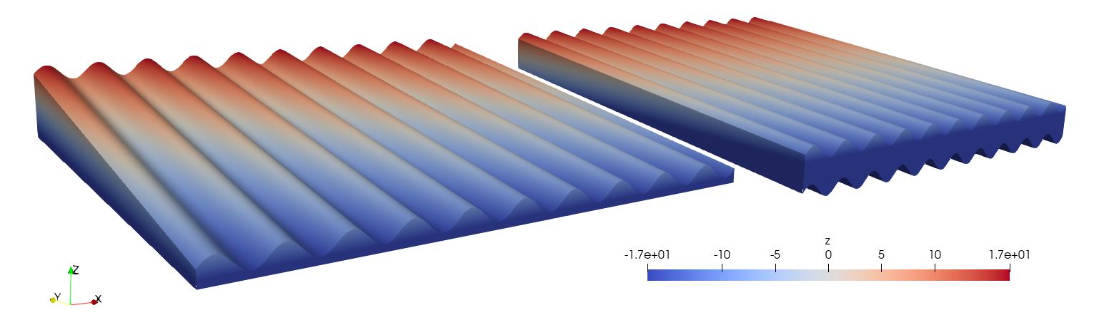
Figure 19 The resulting mesh using either the same topography as the top surface (on the right) or a flat bottom (on the left) for the setup as outlined in flank simulations.

See Figure 19 for the visualization of the different options.

As our computational solution is a surface integral and the interior contributions should cancel out, we can understand the possible repercussion of this predicament. Neither is an accurate representation of reality and from theory we know the effect could be significant. Therefore, the differences need to be investigated and both methods will be used and compared.

Model setup

To compare the two methods, similar model setups as before are used. Again, testing incorporates the subtraction of a flat-terrain domain from the final results. Tests are done on domains with sizes of \(250\times250\times10\) and \(250\times250\times20\) meter, adhering previously establish tresholds for the amount of elements.

Results

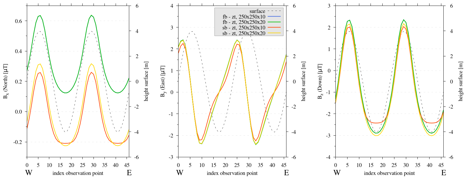
Figure 20 Three subplots depicting the components of the computed magnetic field B for the depth experiments. The numbers in the key relate to the length of each side of the domain (Lx_Ly_Lz). Please note, the y-axis varies between each subplot.

In Figure 20, we observe that the solution of subtraction a zero topography method does not produce adequate results if the same topography is used at the bottom, which is to be expected, as in this setup the bottom surface for the zero topography domain and regular run are not identical.

Reproduce

Steps to reproduce the results and figures for synthetic topography

Please note basic setup in Installation.

1. In MTE.py, modify benchmark attribution to 5, and make sure the right setup is used:

   Code 182 /main/MTE.py

   benchmark = '5'
   
   compute_vi = False  # This includes the volume integral computation by Gaussian quadrature, see
                        # documentation, possible for all setups apart from DEM (-1).
   if compute_vi:
      nqdim = 6  # Number of quadrature points, see documentation.
   
   ## ONLY BENCHMARK = -1 (DEM) & BENCHMARK = 5 (FLANKSIM) ##
   flat_bottom = False  # If True, a flat bottom is generated at the lower surface of the domain.
                       # Please see documentation, as the specific setup of this feature is different
                       # for the flank simulations and the DEM test.
   remove_zerotopo = True  # Setup run 2 times: 1st time, zero topography setup: xy coordinates
                           # of the observation points the same, but zerotopo domain and obs path
                           # shifted to average height DEM. 2nd time, "regular" run with topography.
                           # final results are 2nd run - 1 st run values. Run time can be improved,
                           # if 1st run is done with less el (and cuboid function), yet to be done.
   
   ## ONLY BENCHMARK = 5 (FLANKSIM) ##
   subbench = 'south'  # 'south', 'east', 'north', 'west', input parameters imported from flanksim
              # have priority over any choice made here. So if this is used, make sure to
              # comment out the import line in section below!
   global_run = False
   

2. Run two same bottom setups & move files (not included lines same as before)

   Code 183 /main/MTE.py # Domain settings Lx, Ly, Lz = 250, 250, 10 nelx, nely, nelz = int(Lx * 1.5), int(Ly * 1.5), 10 Mx0, My0, Mz0 = 0, 4.085, -6.29 #Lx, Ly, Lz = 50, 50, 120 #nelx, nely, nelz = 10, 10, 10 # Synthetic topography settings wavelength = 25 A = 6 af = 6

   Code 184 /main/MTE.py # Domain settings Lx, Ly, Lz = 250, 250, 20 nelx, nely, nelz = int(Lx * 1.5), int(Ly * 1.5), 10 Mx0, My0, Mz0 = 0, 4.085, -6.29 #Lx, Ly, Lz = 50, 50, 120 #nelx, nely, nelz = 10, 10, 10 # Synthetic topography settings wavelength = 25 A = 6 af = 6

   Code 185 /main/ (runtime: ~1 hr, ~1 hr)

   python3 -u MTE.py | tee log.txt
   

   Code 186 /main/ mkdir -p flanksim_parameters/south/ztr/250_250_10_sb && mv log.txt *.vtu *.ascii $_

   Code 187 /main/ mkdir -p flanksim_parameters/south/ztr/250_250_20_sb && mv log.txt *.vtu *.ascii $_

3. Go to directory & plot to visualize

   Code 188 /main/

   cd flanksim_parameters/
   

   Code 189 /main/flanksim_parameters/

   gnuplot plot_script_sb.p
   

Conclusions

The results from the parameter tests as desciribed above, allow for establishment of several tresholds for optimized model setups:

1. The amount of elements in the z-direction is irrelevant and will be maintained at ten.

2. The amount of elements in the xy-direction for synthetic topography should be at least 1.5 elements per meter (at a height of 1 meter above the surface).

3. The spatial extent of the domain needs to be at least \(250\times250m\) to avoid a significant edge effect on a central measurement path (of ~:math:50m).

4. Extending the depth and spatial extent has a proportional impact on the magnitude of the \(B_z\) and \(B_x\) components.

   • Increasing the depth for a domain leads to enlargement of the edge effect, so the depth of the domain should remain considerably less than the spatial dimension.

   • To remove the domain related variations, one can subtract the values computed over a flat topography domain from the observed results. We recommend implementing a flat boundary surface at a consistent depth beneath the lowest topographical point within the domain. The thickness of this “zero topography” domain should be calibrated to match that beneath the observation path within the topographic domain.

Footnotes

1

To avoid redundancy, in this section we outline one setup for each of tests done, if repeated tests are done with different setups, the rest of the model setups are located in side by side code snippets. To be able to fully reproduce the figures, all these setups are required.