Benchmarks
Assumption that the contribution of an element can be represented by a single dipole “far” away from source (see Governing equations).
Shape / orientation of the magnetic field outside source body, verifying rotation of vector components in translation from original
facmagFORTRAN77 subroutine [Blakely, 1995], to current function embedded in MTE.Assumption that volume elements are small enough and distance to
Pis large enough (see Computational approach).Solving spatial problem with introduction of a small distance (\(\epsilon\)) suffices.
support.compute_analytical_solution(). All benchmarks outlined here do not require modification of the z-coordinate of nodes on the top and bottom surfaces and, consequently, do not call for a setup with additional triangles (see Computational approach). Therefore, unless otherwise specified, the function magnetostatics.compute_B_surface_integral_cuboid() computes the contribution of each element to the magnetic field strength \(\mathbf{B}\) for all benchmarks.Benchmark 1: a single dipole
Analytical solution
Model setup
Results
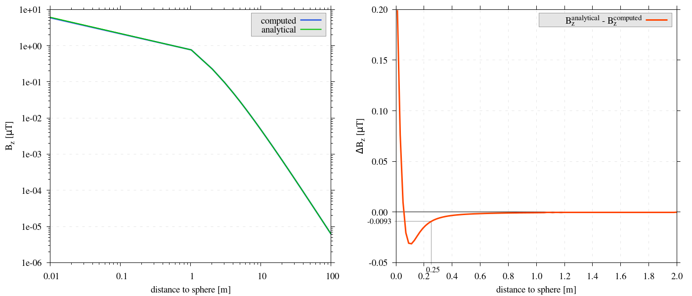
Figure 2 On the left, analytical solution for a single dipole and computed values at increasing distance from surface of a sphere. On the right, the difference between analytical solution for a single dipole and computed values at increasing distance from surface of a sphere. Both show an excellent match of the computed and analytical values, even at close proximity to the surface. At \(0.25m\) the error remains approximately \(\sim \lvert 0.01 \rvert \mu T\).
Reproduce
Steps to reproduce the results and figures
Please note basic setup in Installation
In
MTE.py, modify benchmark attribution to1:49benchmark = '1'Run “zoomed” setup & rename/move files
 88
 89
 90
 91
 92
 93
 94
 95
 96
 97
 98
 99
100
101
102
103
104
105
106
107
108
109
110
111
112
113
114
115
116
if benchmark == '1':
    # General settings
    remove_zerotopo = False
    compute_analytical = True
    do_spiral_measurements = False
    do_path_measurements = False

    # Domain settings
    Lx, Ly, Lz = 2, 2, 2  # Length of the domain in each direction.
    nelx, nely, nelz = 100, 100, 100  # Amount of elements in each direction.
    Mx0, My0, Mz0 = 0, 0, 7.5  # Magnetization [A/m], do not change Mx0 and My0.

    # Sphere settings
    sphere_R = 1  # Radius of the sphere.
    sphere_xc, sphere_yc, sphere_zc = Lx / 2, Ly / 2, -Lz / 2  # Center position of the sphere.

    # Line measurement settings
    do_line_measurements = True  # Do computations along a observation line (path).
    line_nmeas = 100  # Amount of observation points.
    xstart, xend = Lx / 2, Lx / 2  # x-coordinates of start and end of observation path.
    ystart, yend = Ly / 2, Ly / 2  # y-coordinates "".
    zstart, zend = 0.01, 2 # Zoomed setup.
    #zstart, zend = 0.01, 100  # Non-zoomed setup.

    # Plane measurement settings
    do_plane_measurements = False  # Do computations on a observation plane.
    plane_nnx, plane_nny = 3, 3  # Amount of observation points in each direction.
    plane_x0, plane_y0, plane_z0 = -Lx / 2, -Ly / 2, 1
    plane_Lx, plane_Ly = 2 * Lx, 2 * Ly  # Length of observation plane in each direction.
python3 -u MTE.py | tee log.txt
mkdir -p benchmarks/benchmark_1/results_zoom && mv log.txt *.vtu *.ascii $_
Run regular setup & move files
104
105
106
107
108
109
110
# Line measurement settings
do_line_measurements = True  # Do computations along a observation line (path).
line_nmeas = 100  # Amount of observation points.
xstart, xend = Lx / 2, Lx / 2  # x-coordinates of start and end of observation path.
ystart, yend = Ly / 2, Ly / 2  # y-coordinates "".
#zstart, zend = 0.01, 2 # Zoomed setup.
zstart, zend = 0.01, 100  # Non-zoomed setup.
python3 -u MTE.py | tee log.txt
mv log.txt *.vtu *.ascii benchmarks/benchmark_1/
Go to directory & plot
cd benchmarks/benchmark_1
gnuplot plot_script_B1.p
python3 plot_script_B1.py
Benchmark 2: internal cancellation
Analytical solution
Model setup

Figure 3 Visualization of different model setups by cross sectional (z-y) planes trough middle of each domain. On the left the undeformed base domain, in the middle deformation setup (1), where perturbations within a range of \([-0.1:0.1m]\) are introduced to the z-coordinates of the internal nodes of the domain. On the right deformation setup (2), where the same perturbations are repeated, additionally, the aspect ratio of elements are increased.
A random value between \(-0.1\) and \(0.1m\) is added to the z coordinates of internal nodes.
In addition to situation (1), the aspect ratio of elements is significantly increased, with each element’s dimension now \(5\times1\times0.2m\).
Results
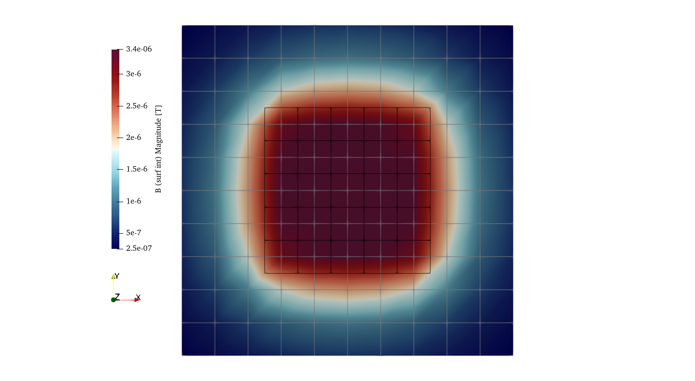
Figure 4 The magnetic field strength \(\mathbf{B}\) on a plane \(1m\) above the surface of a box with a spatial extent that is twice as large as the (undeformed) domain beneath. Black lines denote the domain edges, while the grey lines connect the observation points on the plane. The observed pattern reveals the extent of the magnetization of the cuboid domain, rapidly decreasing with distance from the domain. These results provided the base for further testing in this benchmark.
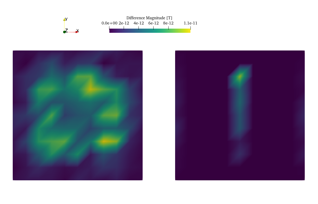
Figure 5 Difference between Figure 4 and results from the deformed domain setups. The left side depicts the variance between deformation setup (1) and the base, while the right side shows the difference of deformation setup (2) relative to the base. Notably, the errors in both deformation setups are minimal.
Reproduce
Steps to reproduce the results and figures
Please note basic setup in Installation
In
MTE.py, modify benchmark attribution to2a:49benchmark = '2a'Run base setup & rename/move files
120
121
122
123
124
125
126
127
128
129
130
131
132
133
134
135
136
137
138
139
140
141
142
143
if benchmark == '2a':
   # General settings
   remove_zerotopo = False
   compute_analytical = False
   do_spiral_measurements = False
   do_path_measurements = False

   # Domain settings
   Lx, Ly, Lz = 10, 10, 10
   nelx, nely, nelz = 5, 5, 5
   Mx0, My0, Mz0 = 0, 0, 7.5  # Magnetization [A/m].

   # Plane measurement settings
   do_plane_measurements = True
   plane_nnx, plane_nny = 11, 11
   plane_x0, plane_y0, plane_z0 = -Lx / 2, -Ly / 2, 1
   plane_Lx, plane_Ly = 2 * Lx, 2 * Ly

   # Line measurement settings
   do_line_measurements = False
   line_nmeas = 47
   xstart, xend = 0.23 + ((Lx - 50) / 2), 49.19 + ((Ly - 50) / 2)
   ystart, yend = Ly / 2 - 0.221, Ly / 2 - 0.221
   zstart, zend = 1, 1  # 1m above surface.
python3 -u MTE.py | tee log.txt
mkdir -p benchmarks/benchmark_2/d0 && mv log.txt *.vtu *.ascii $_
In
MTE.py, modify benchmark attribution to2b:49benchmark = '2b'Run deformation setup (1) & move files
147
148
149
150
151
152
153
154
155
156
157
158
159
160
161
162
163
164
165
166
if benchmark == '2b':
   # General settings
   remove_zerotopo = False
   compute_analytical = False
   do_spiral_measurements = False
   do_path_measurements = False
   do_line_measurements = False

   # Domain settings
   Lx, Ly, Lz = 10, 10, 10
   nelx, nely, nelz = 5, 5, 5
   #nelx, nely, nelz = 2, 10, 50
   Mx0, My0, Mz0 = 0, 0, 7.5
   dz = 0.1  # Amplitude random for perturbations in domain.

   # Plane measurement settings
   do_plane_measurements = True
   plane_nnx, plane_nny = 11, 11
   plane_x0, plane_y0, plane_z0 = -Lx / 2, -Ly / 2, 1
   plane_Lx, plane_Ly = 2 * Lx, 2 * Ly
python3 -u MTE.py | tee log.txt
mkdir -p benchmarks/benchmark_2/d0_1 && mv log.txt *.vtu *.ascii $_
Run deformation setup (2) & move files
155
156
157
158
159
160
# Domain settings
Lx, Ly, Lz = 10, 10, 10
#nelx, nely, nelz = 5, 5, 5
nelx, nely, nelz = 2, 10, 50
Mx0, My0, Mz0 = 0, 0, 7.5
dz = 0.1  # Amplitude random for perturbations in domain.
python3 -u MTE.py | tee log.txt
mkdir -p benchmarks/benchmark_2/d0_1_2_10_50 && mv log.txt *.vtu *.ascii $_
Go to directory & use paraview or plotting to visualize
cd benchmarks/benchmark_2
paraview --state=plot_result_b2_final.pvsm
gnuplot plot_script_B2.p
python3 plot_script_B2.py
Benchmark 3: a magnetized sphere
Analytical solution
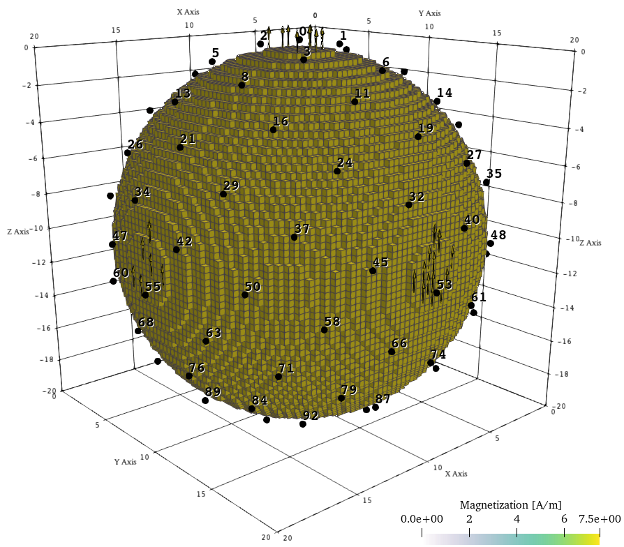
Figure 6 Visualization of the model setup with numbering along Fibonacci spiral for uniform distribution above the tessellated sphere. The numbering sequence begins at the top of the sphere and proceeds downward in a counterclockwise spiral. The magnetization is assigned to any elements within the spherical domain, and aligned with the z-axis.
Model setup
Results
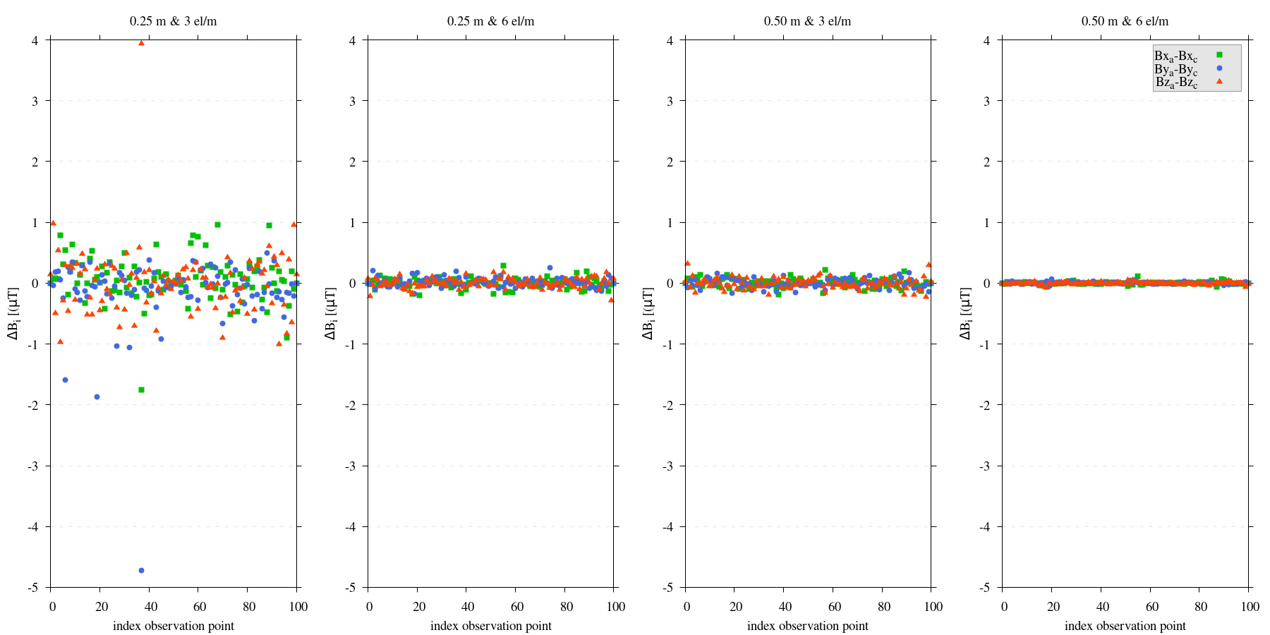
Figure 7 Comparative analysis of the analytical solution versus computed values at \(101\) distinct observation points, located either \(0.25m\) or \(0.5m\) above a sphere’s surface. The resolutions tested are \(3\) or \(6\) elements per meter (\(el/m\)). It is demonstrated that increasing the number of elements substantially reduces the discrepancy between analytical and computed values.
Reproduce
Steps to reproduce the results and figures
Please note basic setup in Installation
In
MTE.py, modify benchmark attribution to3:49benchmark = '3'Run 25cm above setup & rename/move files
170
171
172
173
174
175
176
177
178
179
180
181
182
183
184
185
186
187
188
189
190
191
192
193
194
195
196
197
if benchmark == '3':
   # General settings
   remove_zerotopo = False
   compute_analytical = True
   do_line_measurements = False
   do_path_measurements = False

   # Domain settings
   Lx, Ly, Lz = 20, 20, 20
   nelx, nely, nelz = 60, 60, 60  # 3 el/m.
   #nelx, nely, nelz = 120, 120, 120  # 6 el/m.
   Mx0, My0, Mz0 = 0, 0, 7.5

   # Sphere settings
   sphere_R = 10  # Do not change, or change radius_spiral as well.
   sphere_xc, sphere_yc, sphere_zc = Lx / 2, Ly / 2, -Lz / 2

   # Spiral measurement settings
   do_spiral_measurements = True
   npts_spiral = 101  # keep odd
   radius_spiral = 1.025 * sphere_R  # 25 cm above surface sphere.
   #radius_spiral = 1.05 * sphere_R  # 50 cm above surface sphere.

   # Plane measurement settings
   do_plane_measurements = False
   plane_nnx, plane_nny = 30, 30
   plane_x0, plane_y0, plane_z0 = -Lx / 2, -Ly / 2, 0.5
   plane_Lx, plane_Ly = 2 * Lx, 2 * Ly
python3 -u MTE.py | tee log.txt
mkdir -p benchmarks/benchmark_3/0_25_above && mv log.txt *.vtu *.ascii $_
Run 25cm above setup with double amount of elements & rename/move files
177
178
179
180
181
182
183
184
185
186
187
188
189
190
191
# Domain settings
Lx, Ly, Lz = 20, 20, 20
#nelx, nely, nelz = 60, 60, 60  # 3 el/m.
nelx, nely, nelz = 120, 120, 120  # 6 el/m.
Mx0, My0, Mz0 = 0, 0, 7.5

# Sphere settings
sphere_R = 10  # Do not change, or change radius_spiral as well.
sphere_xc, sphere_yc, sphere_zc = Lx / 2, Ly / 2, -Lz / 2

# Spiral measurement settings
do_spiral_measurements = True
npts_spiral = 101  # keep odd
radius_spiral = 1.025 * sphere_R  # 25 cm above surface sphere.
#radius_spiral = 1.05 * sphere_R  # 50 cm above surface sphere.
python3 -u MTE.py | tee log.txt
mkdir -p benchmarks/benchmark_3/0_25_2_above && mv log.txt *.vtu *.ascii $_
Run 50cm above setup & rename/move files
177
178
179
180
181
182
183
184
185
186
187
188
189
190
191
# Domain settings
Lx, Ly, Lz = 20, 20, 20
nelx, nely, nelz = 60, 60, 60  # 3 el/m.
#nelx, nely, nelz = 120, 120, 120  # 6 el/m.
Mx0, My0, Mz0 = 0, 0, 7.5

# Sphere settings
sphere_R = 10  # Do not change, or change radius_spiral as well.
sphere_xc, sphere_yc, sphere_zc = Lx / 2, Ly / 2, -Lz / 2

# Spiral measurement settings
do_spiral_measurements = True
npts_spiral = 101  # keep odd
#radius_spiral = 1.025 * sphere_R  # 25 cm above surface sphere.
radius_spiral = 1.05 * sphere_R  # 50 cm above surface sphere.
python3 -u MTE.py | tee log.txt
mkdir -p benchmarks/benchmark_3/0_5_above && mv log.txt *.vtu *.ascii $_
Run 50cm above setup with double amount of elements & rename/move files
177
178
179
180
181
182
183
184
185
186
187
188
189
190
191
# Domain settings
Lx, Ly, Lz = 20, 20, 20
#nelx, nely, nelz = 60, 60, 60  # 3 el/m.
nelx, nely, nelz = 120, 120, 120  # 6 el/m.
Mx0, My0, Mz0 = 0, 0, 7.5

# Sphere settings
sphere_R = 10  # Do not change, or change radius_spiral as well.
sphere_xc, sphere_yc, sphere_zc = Lx / 2, Ly / 2, -Lz / 2

# Spiral measurement settings
do_spiral_measurements = True
npts_spiral = 101  # keep odd
#radius_spiral = 1.025 * sphere_R  # 25 cm above surface sphere.
radius_spiral = 1.05 * sphere_R  # 50 cm above surface sphere.
python3 -u MTE.py | tee log.txt
mkdir -p benchmarks/benchmark_3/0_5_2_above && mv log.txt *.vtu *.ascii $_
Go to directory & plot
cd benchmarks/benchmark_3
gnuplot plot_script_B3.p
python3 plot_script_B3.py
(OPTIONAL) Use paraview to visualize model setups
tee ./0_5_above/model_setup.pvsm ./0_5_2_above/model_setup.pvsm ./0_25_2_above/model_setup.pvsm ./0_25_above/model_setup.pvsm < ./model_setup.pvsm >/dev/null
paraview --state=0_5_2_above/model_setup.pvsm
paraview --state=0_5_above/model_setup.pvsm
paraview --state=0_25_above/model_setup.pvsm
paraview --state=0_25_2_above/model_setup.pvsm
Benchmark 4: a prismatic body
Analytical solution
Model setup
magnetostatics.compute_B_surface_integral_cuboid() would suffice. Nonetheless, to validate our proposed solution (see support.shift_observation_points_edge()) for additional singularities on diagonals of domain elements, function magnetostatics.compute_B_surface_integral_wtopo() is still utilized.Results
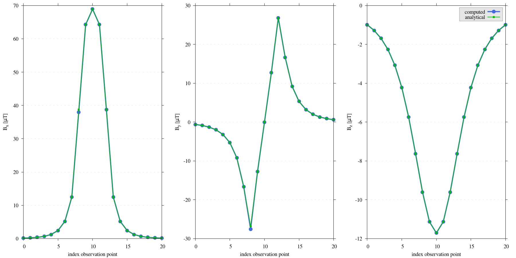
Figure 8 Comparison of magnetic field components \(\mathbf{B_x}\), \(\mathbf{B_y}\), \(\mathbf{B_z}\) for the prismatic body. As observation site location are displaced from [Ren et al., 2017], the x-axis now refers to index relating to the observation point rather than distance. The computed values of our study match those of [Ren et al., 2019].
Discussion
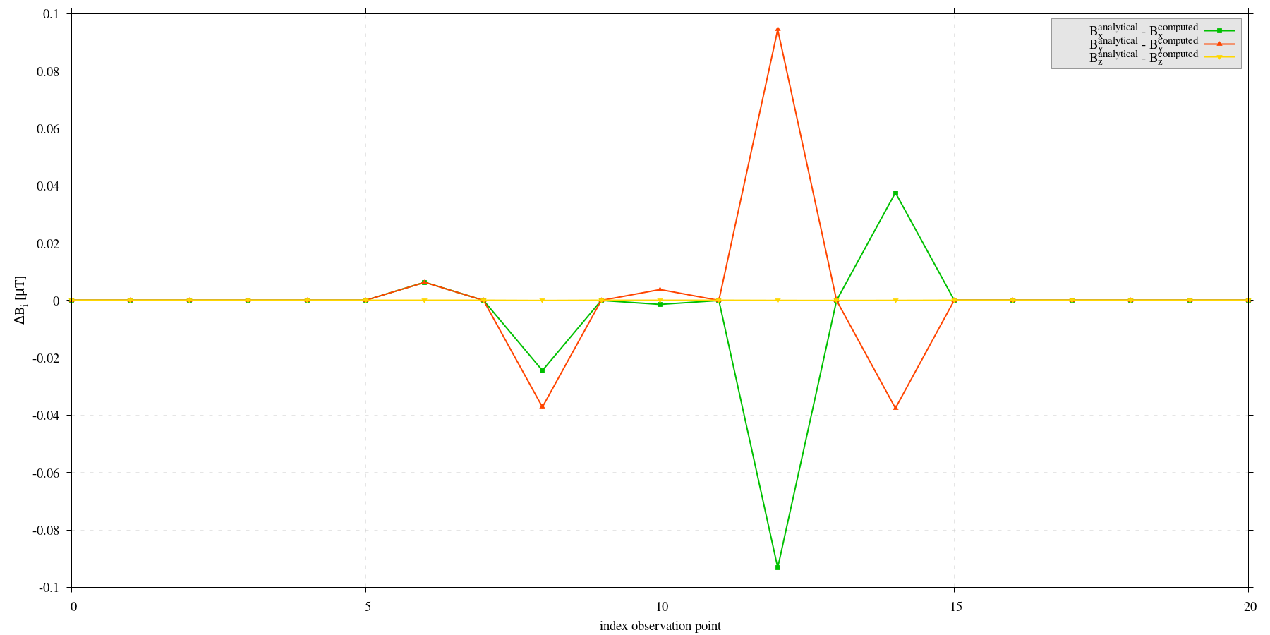
Figure 9 Comparison of magnetic field components \(\mathbf{B_x}\), \(\mathbf{B_y}\), \(\mathbf{B_z}\) for the prismatic body. As observation site location are displaced from [Ren et al., 2017], the x-axis now refers to index relating to the observation point rather than distance. The differences are small compared to the absolute values depicted in the previous graph.
Reproduce
Steps to reproduce the results and figures
Please note basic setup in Installation
In
MTE.py, modify benchmark attribution to4:49benchmark = '4'Run setup & rename/move files
201
202
203
204
205
206
207
208
209
210
211
212
213
214
215
216
217
218
219
220
221
222
223
224
225
226
227
if benchmark == '4':
   # General settings
   remove_zerotopo = False
   compute_analytical = False
   do_plane_measurements = False
   do_spiral_measurements = False
   do_path_measurements = False

   # Domain settings
   Lx, Ly, Lz = 10, 10, 10
   nelx, nely, nelz = int(Lx), int(Ly), 10
   Mx0, My0, Mz0 = 0, 0, 200

   # Line measurement settings
   do_line_measurements = True
   line_nmeas = 21
   xstart, xend = 6, 6
   ystart, yend = -25, 25
   zstart, zend = 0, 0

   # Reading in values from Ren.
   pathfile = 'sites/B.dat'
   with open(pathfile, 'r') as path:
        lines_path = path.readlines()
   BxB4, ByB4, BzB4  = np.zeros((3, len(lines_path)), dtype=np.float64)  # Bx, By, Bz from Ren.
   data = np.array([list(map(float, line.split())) for line in lines_path])
   BxB4, ByB4, BzB4 = data[:, 0], data[:, 1], data[:, 2]
python3 -u MTE.py | tee log.txt
mv log.txt *.vtu *.ascii benchmarks/benchmark_4/
Go to directory & plot
cd benchmarks/benchmark_4
gnuplot plot_script_B4.p
python3 plot_script_B4.py
Note
If the resulted difference is unsatisfactory, see discussion section and repeat run to randomly generate new observation point for the model.